.男篮世界杯预选赛中国vs黎巴嫩『wn4.com』咪咕世界杯营销方案.w6n2c9o.2022年11月29日5时52分2秒.yeyo8yaka

SearchAdvancedHelp

(0.006 seconds)

11—20 of 814 matching pages

11: 28.6 Expansions for Small $q$

… ►For more details on these expansions and recurrence relations for the coefficients see Frenkel and Portugal (2001, §2). ►The coefficients of the power series of $a_{2n}\left(q\right)$, $b_{2n}\left(q\right)$ and also $a_{2n+1}\left(q\right)$, $b_{2n+1}\left(q\right)$ are the same until the terms in $q^{2n-2}$ and $q^{2n}$, respectively. … ►Here $j=1$ for $a_{2n}\left(q\right)$, $j=2$ for $b_{2n+2}\left(q\right)$, and $j=3$ for $a_{2n+1}\left(q\right)$ and $b_{2n+1}\left(q\right)$. … ►where $k$ is the unique root of the equation $2E\left(k\right)=K\left(k\right)$ in the interval $(0,1)$, and $k^{\prime }=\sqrt{1-k^2}$. … ►For more details on these expansions and recurrence relations for the coefficients see Frenkel and Portugal (2001, §2). …

12: 25.20 Approximations

… ►

Cody et al. (1971) gives rational approximations for $\zeta \left(s\right)$ in the form of quotients of polynomials or quotients of Chebyshev series. The ranges covered are $0.5\le s\le 5$, $5\le s\le 11$, $11\le s\le 25$, $25\le s\le 55$. Precision is varied, with a maximum of 20S.

►

Piessens and Branders (1972) gives the coefficients of the Chebyshev-series expansions of $s\zeta \left(s+1\right)$ and $\zeta \left(s+k\right)$, $k=2,3,4,5,8$, for $0\le s\le 1$ (23D).

►

Luke (1969b, p. 306) gives coefficients in Chebyshev-series expansions that cover $\zeta \left(s\right)$ for $0\le s\le 1$ (15D), $\zeta \left(s+1\right)$ for $0\le s\le 1$ (20D), and $\ln \xi \left(\frac{1}{2}+\mathrm{i}x\right)$ (§25.4) for $-1\le x\le 1$ (20D). For errata see Piessens and Branders (1972).

►

Morris (1979) gives rational approximations for ${\mathrm{Li}}_2\left(x\right)$ (§25.12(i)) for $0.5\le x\le 1$. Precision is varied with a maximum of 24S.

►

Antia (1993) gives minimax rational approximations for $\mathrm{\Gamma }\left(s+1\right)F_s(x)$, where $F_s(x)$ is the Fermi–Dirac integral (25.12.14), for the intervals and , with $s=-\frac{1}{2},\frac{1}{2},\frac{3}{2},\frac{5}{2}$. For each $s$ there are three sets of approximations, with relative maximum errors ${10}^{-4},{10}^{-8},{10}^{-12}$.

13: 24.20 Tables

… ►Abramowitz and Stegun (1964, Chapter 23) includes exact values of ${\sum }_{k=1}^m{k}^n$, $m=1(1)100$, $n=1(1)10$; ${\sum }_{k=1}^{\mathrm{\infty }}{k}^{-n}$, ${\sum }_{k=1}^{\mathrm{\infty }}{(-1)}^{k-1}{k}^{-n}$, ${\sum }_{k=0}^{\mathrm{\infty }}{(2k+1)}^{-n}$, $n=1,2,\mathrm{\dots }$, 20D; ${\sum }_{k=0}^{\mathrm{\infty }}{(-1)}^k{(2k+1)}^{-n}$, $n=1,2,\mathrm{\dots }$, 18D. ►Wagstaff (1978) gives complete prime factorizations of $N_n$ and $E_n$ for $n=20(2)60$ and $n=8(2)42$, respectively. In Wagstaff (2002) these results are extended to $n=60(2)152$ and $n=40(2)88$, respectively, with further complete and partial factorizations listed up to $n=300$ and $n=200$, respectively. ►For information on tables published before 1961 see Fletcher et al. (1962, v. 1, §4) and Lebedev and Fedorova (1960, Chapters 11 and 14).

14: 27.2 Functions

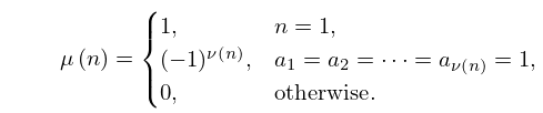
… ►where $p_1,p_2,\mathrm{\dots },p_{\nu \left(n\right)}$ are the distinct prime factors of $n$, each exponent $a_r$ is positive, and $\nu \left(n\right)$ is the number of distinct primes dividing $n$. … ►The $\varphi \left(n\right)$ numbers $a,a^2,\mathrm{\dots },a^{\varphi \left(n\right)}$ are relatively prime to $n$ and distinct (mod $n$). …It is the special case $k=2$ of the function $d_k\left(n\right)$ that counts the number of ways of expressing $n$ as the product of $k$ factors, with the order of factors taken into account. … ►

27.2.12

ⓘ

Defines:

$\mu \left(n\right)$: Möbius function

Symbols:

$\nu \left(n\right)$: number of distinct primes dividing a number, $n$: positive integer and $a$: primitive root

A&S Ref:

24.3.1 I.A

Permalink:

http://dlmf.nist.gov/27.2.E12

Encodings:

pMML, png, TeX

See also:

Annotations for §27.2(i), §27.2 and Ch.27

… ►

Table 27.2.2: Functions related to division.

► ►►►

$n$	$\varphi \left(n\right)$	$d\left(n\right)$	$\sigma \left(n\right)$	$n$	$\varphi \left(n\right)$	$d\left(n\right)$	$\sigma \left(n\right)$	$n$	$\varphi \left(n\right)$	$d\left(n\right)$	$\sigma \left(n\right)$	$n$	$\varphi \left(n\right)$	$d\left(n\right)$	$\sigma \left(n\right)$
…
11	10	2	12	24	8	8	60	37	36	2	38	50	20	6	93
…

►

15: Bibliography

… ►

Asymptotic expansions of spheroidal wave functions. J. Math. Phys. Mass. Inst. Tech. 28, pp. 195–199.

ⓘ

External Links:

MathReview (J. G. van der Corput), ZentralBlatt

Referenced by:

§30.9(iii).

Encodings:

BibTeX

… ►

Complex Analysis: An Introduction of the Theory of Analytic Functions of One Complex Variable. 2nd edition, McGraw-Hill Book Co., New York.

ⓘ

Notes:

A third edition was published in 1978 by McGraw-Hill, New York.

External Links:

MathReview (P. Lelong), ZentralBlatt

Referenced by:

§1.9(iii), §23.18.

Encodings:

BibTeX

… ►

On the zeros of confluent hypergeometric functions. III. Characterization by means of nonlinear equations. Lett. Nuovo Cimento (2) 29 (11), pp. 353–358.

ⓘ

External Links:

ISSN 0024-1318, MathReview (James M. Horner)

Referenced by:

§13.9(i).

Encodings:

BibTeX

… ►

Normal forms of functions in the neighborhood of degenerate critical points. Uspehi Mat. Nauk 29 (2(176)), pp. 11–49 (Russian).

ⓘ

Notes:

Collection of articles dedicated to the memory of Ivan Georgievič Petrovskiĭ (1901–1973), I. In Russian. English translation: Russian Math. Surveys, 29(1974), no. 2, pp. 10–50.

External Links:

Document, MathReview (G. R. Belickii), ZentralBlatt

Referenced by:

§36.2(i).

Encodings:

BibTeX

… ►

Some basic hypergeometric extensions of integrals of Selberg and Andrews. SIAM J. Math. Anal. 11 (6), pp. 938–951.

ⓘ

External Links:

ISSN 0036-1410, Document, MathReview (W. A. Al-Salam), ZentralBlatt

Referenced by:

§17.13, §17.13.

Encodings:

BibTeX

…

16: Bibliography E

… ►

The penetration of a potential barrier by electrons. Phys. Rev. 35 (11), pp. 1303–1309.

ⓘ

External Links:

Document, ZentralBlatt

Referenced by:

§15.18.

Encodings:

BibTeX

… ►

Interlacing properties of the zeros of Bessel functions. Atti Sem. Mat. Fis. Univ. Modena XLII (2), pp. 525–529.

ⓘ

External Links:

ISSN 0041-8986, MathReview (Evangelos Ifantis), ZentralBlatt

Referenced by:

§10.21(i).

Encodings:

BibTeX

… ►

Higher Transcendental Functions. Vol. II. McGraw-Hill Book Company, Inc., New York-Toronto-London.

ⓘ

Notes:

Reprinted by Robert E. Krieger Publishing Co. Inc., 1981. Table errata: Math. Comp. v. 41 (1983), no. 164, p. 778, v. 36 (1981), no. 153, p. 315, v. 30 (1976), no. 135, p. 675, v. 29 (1975), no. 130, p. 670, v. 26 (1972), no. 118, p. 598, v. 25 (1971), no. 113, p. 199, v. 24 (1970), no. 109, p. 239, v. 17 (1963), no. 84, p. 485.

External Links:

MathReview (E. T. Copson), ZentralBlatt

Referenced by:

§10.22(iv), §10.22(vi), §10.23(iii), §10.23(iii), §10.23(iv), §10.32(i), §10.32(iii), §10.32(iv), §10.43(iv), §10.43(vi), §10.44(iv), §10.60(iv), §10.9(i), §10.9(iii), §10.9(iv), §11.10(vi), §11.4(i), Ch.11, §12.12, §12.12, §12.13(i), §12.5(iv), Ch.12, §18.16(vi), (18.17.21_1), §18.17(iv), §18.17(i), §18.17(viii), (18.35.1), (18.35.2), (18.35.4_5), §18.35(i), (18.5.11_1), (18.5.11_3), §18.5(ii), §18.9(iii), §19.1, §19.10(i), §19.14(ii), (19.25.40), §19.25(vi), §19.5, §19.7(ii), §19.9(i), Ch.19, §20.9(i), §22.15(ii), §23.6(iv), Ch.23, §8.13(i), §8.14, §8.3(i), §8.4, §8.6(iii), §8.7, Ch.8, Notations P, Notations P.

Encodings:

BibTeX

… ►

Painlevé transcendent describes quantum correlation function of the $XXZ$ antiferromagnet away from the free-fermion point. J. Phys. A 29 (17), pp. 5619–5626.

ⓘ

External Links:

ISSN 0305-4470, Document, MathReview (Estelle L. Basor), ZentralBlatt

Referenced by:

§32.16.

Encodings:

BibTeX

… ►

Institutiones Calculi Integralis. Opera Omnia (1), Vol. 11, pp. 110–113.

ⓘ

Referenced by:

§25.12(i).

Encodings:

BibTeX

…

17: Bibliography L

… ►

Eine Verallgemeinerung der Sphäroidfunktionen. Arch. Math. 11, pp. 29–39.

ⓘ

External Links:

ISSN 0003-9268, Document, MathReview (M. J. O. Strutt), ZentralBlatt

Referenced by:

§30.12.

Encodings:

BibTeX

… ►

Note sur la fonction $𝔎(w,x,s)={\sum }_{k=0}^{\mathrm{\infty }}\frac{e^{2k\pi ix}}{{(w+k)}^s}$ . Acta Math. 11 (1-4), pp. 19–24 (French).

ⓘ

External Links:

ISSN 0001-5962, Document, MathReview Entry, ZentralBlatt

Referenced by:

§25.14(i), Notations K.

Encodings:

BibTeX

… ►

Algorithm 244: Fresnel integrals. Comm. ACM 7 (11), pp. 660–661.

ⓘ

Notes:

Includes Algol program, maximum accuracy 12D.

External Links:

ISSN 0001-0782, Document

Referenced by:

§7.25(iv).

Encodings:

BibTeX

… ►

On the theory of Painlevé’s third equation. Differ. Uravn. 3 (11), pp. 1913–1923 (Russian).

ⓘ

Notes:

In Russian. English translation: Differential Equations 3(11), pp. 994–999

External Links:

MathReview (Z. Nehari), ZentralBlatt

Referenced by:

§32.10(iii), §32.8(iii), §32.9(i), §32.9(ii).

Encodings:

BibTeX

… ►

Algorithms for rational approximations for a confluent hypergeometric function. Utilitas Math. 11, pp. 123–151.

ⓘ

External Links:

MathReview (F. Gotze), ZentralBlatt

Referenced by:

§13.31(iii).

Encodings:

BibTeX

…

18: 26.12 Plane Partitions

… ►The number of self-complementary plane partitions in $B(2r,2s,2t)$ is …in $B(2r+1,2s,2t)$ it is …in $B(2r+1,2s+1,2t)$ it is … ►The number of symmetric self-complementary plane partitions in $B(2r,2r,2t)$ is …in $B(2r+1,2r+1,2t)$ it is …

19: 18.8 Differential Equations

… ►

Table 18.8.1: Classical OP’s: differential equations $A(x)f^{\prime \prime }(x)+B(x)f^{\prime }(x)+C(x)f(x)+{\lambda }_{n}f(x)=0$.

► ►►►►►►

#	$f(x)$	$A(x)$	$B(x)$	$C(x)$	${\lambda }_n$
…
9	${\mathrm{e}}^{-\frac{1}{2}{x}^2}{x}^{\alpha +\frac{1}{2}}{L}_n^{(\alpha )}\left(x^2\right)$	$1$	$0$	$-x^2+(\frac{1}{4}-{\alpha }^2)x^{-2}$	$4n+2\alpha +2$
…
11	${\mathrm{e}}^{-n^{-1}x}{x}^{\mathrm{\ell }+1}{L}_{n-\mathrm{\ell }-1}^{(2\mathrm{\ell }+1)}\left(2n^{-1}x\right)$	$1$	$0$	$\frac{2}{x}-\frac{\mathrm{\ell }(\mathrm{\ell }+1)}{x^2}$	$-\frac{1}{n^2}$
12	$H_n\left(x\right)$	$1$	$-2x$	$0$	$2n$
13	${\mathrm{e}}^{-\frac{1}{2}{x}^2}{H}_n\left(x\right)$	$1$	$0$	$-x^2$	$2n+1$
…

►

►Item 11 of Table 18.8.1 yields (18.39.36) for $Z=1$.

20: Bibliography K

… ►

Bernstein, Pick, Poisson and related integral expressions for Lambert $W$ . Integral Transforms Spec. Funct. 23 (11), pp. 817–829.

ⓘ

External Links:

ISSN 1065-2469, Document, Link, MathReview (Ross C. McPhedran), ZentralBlatt

Referenced by:

§4.13.

Encodings:

BibTeX

… ►

Auxiliary table for the incomplete elliptic integrals. J. Math. Physics 27, pp. 11–36.

ⓘ

External Links:

MathReview (S. C. van Veen), ZentralBlatt

Referenced by:

§19.12.

Encodings:

BibTeX

… ►

An extension of Saalschütz’s summation theorem for the series ${}_{r+3}{}^{}F_{r+2}^{}$ . Integral Transforms Spec. Funct. 24 (11), pp. 916–921.

ⓘ

External Links:

ISSN 1065-2469, Document, FullText, MathReview (Christian Lavault), ZentralBlatt

Referenced by:

§16.4(ii), §16.4(ii).

Encodings:

BibTeX

… ►

Algorithm 327: Dilogarithm [S22]. Comm. ACM 11 (4), pp. 270–271.

ⓘ

Notes:

Includes Algol program, maximum accuracy 12D.

External Links:

ISSN 0001-0782, Document

Referenced by:

§25.21(v).

Encodings:

BibTeX

… ►

Clebsch-Gordan coefficients for $\mathrm{SU}(2)$ and Hahn polynomials. Nieuw Arch. Wisk. (3) 29 (2), pp. 140–155.

ⓘ

External Links:

ISSN 0028-9825, MathReview (Jiří Patera), ZentralBlatt

Referenced by:

§18.38(iii).

Encodings:

BibTeX

…