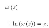
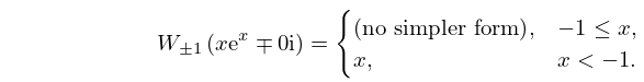
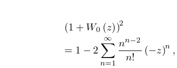
To verify the radius of convergence of the series
(4.13.6) map the plane of onto the plane of
via , where
. Then is
analytic at , and its nearest singularities to the origin are
located at .
Figure 4.13.1 was produced at NIST.
This section has been enlarged. The Lambert -function is multi-valued and we use the notation
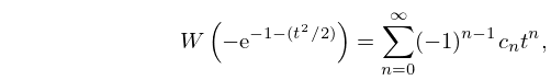
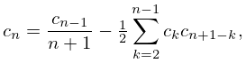
, , for the branches. The original two solutions are identified via
and .
Other changes are the introduction of the Wright -function and tree -function
in (4.13.1_2) and (4.13.1_3), simplification formulas (4.13.3_1) and (4.13.3_2),
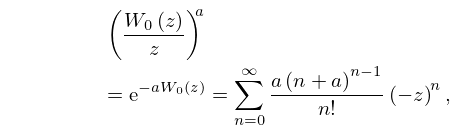
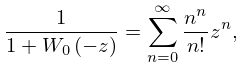
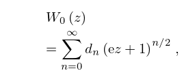
explicit representation (4.13.4_1) for , additional Maclaurin series
(4.13.5_1) and (4.13.5_2), an explicit expansion about the branch point at in
(4.13.9_1), extending the number of terms in asymptotic expansions (4.13.10) and (4.13.11),
and including several integrals and integral representations for Lambert -functions in the end of the section.
Addition (effective with 1.0.9):
The reference to Scott et al. (2014) has been
added at the end of this section.
Addition (effective with 1.0.7):
The references to Scott et al. (2006) and Scott et al. (2013) have been
added at the end of this section.
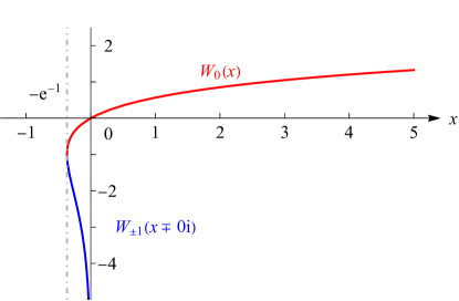
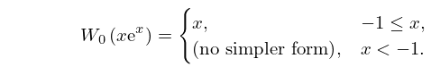
On the -interval there is one real solution, and it is
nonnegative and increasing. On the -interval there are two real
solutions, one increasing and the other decreasing. We call the increasing solution for
which the principal branch and
denote it by .
See Figure 4.13.1.
Figure 4.13.1: Branches , of the Lambert
-function.
Magnify
where .
is a single-valued analytic function on
, real-valued when , and has a square root branch point at .
See (4.13.6) and (4.13.9_1).
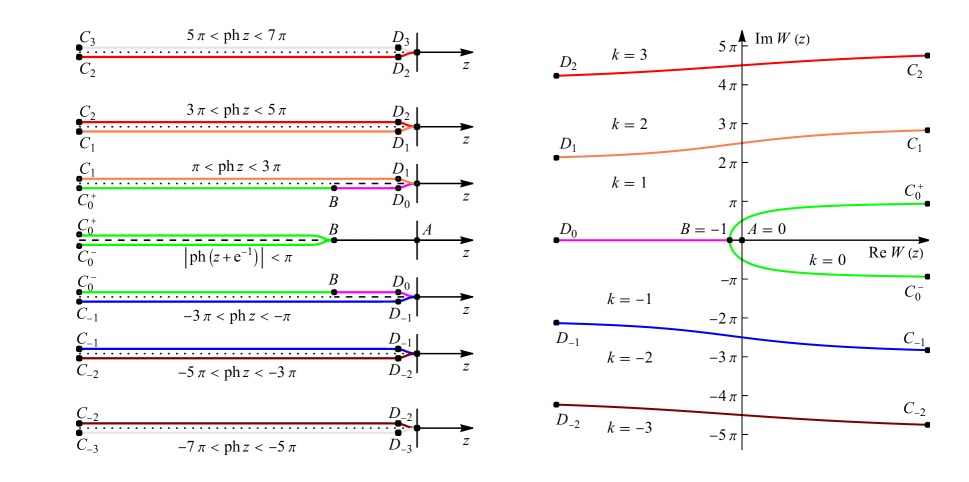
The other branches are single-valued analytic functions on ,
have a logarithmic branch point at , and, in the case , have a square root branch point at respectively.
See Figure 4.13.2.
Figure 4.13.2: The function on the first 5 Riemann sheets.
maps the first Riemann sheet
in the middle of the left-hand side
to the region enclosed by the green curve on the right-hand side;
it maps the Riemann sheet on the left-hand side
to the region enclosed by the pink, green and orange curves on the right-hand side, etc.
Magnify
where .
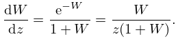
For large enough the series on the right-hand side of (4.13.10) is absolutely convergent to its left-hand side.
In the case of and real the series converges for .
As
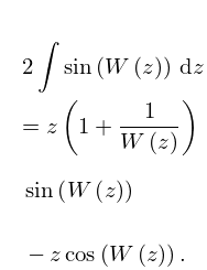
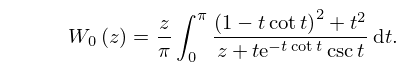
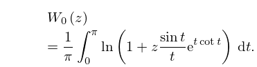
For these and other integral representations of the Lambert -function see Kheyfits (2004), Kalugin et al. (2012) and Mező (2020).
For the foregoing results and further information see
Borwein and Corless (1999), Corless et al. (1996),
de Bruijn (1961, pp. 25–28), Olver (1997b, pp. 12–13), and
Siewert and Burniston (1973).
For a generalization of the Lambert -function connected to the three-body
problem see Scott et al. (2006), Scott et al. (2013) and Scott et al. (2014).

