§25.12 Polylogarithms
Contents
- §25.12(i) Dilogarithms
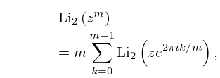
- §25.12(ii) Polylogarithms
- §25.12(iii) Fermi–Dirac and Bose–Einstein Integrals
§25.12(i) Dilogarithms
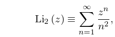
The notation was introduced in Lewin (1981) for a function discussed in Euler (1768) and called the dilogarithm in Hill (1828):
| 25.12.1 | |||
| . | |||
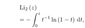
| 25.12.2 | |||
| . | |||
Other notations and names for include (Kölbig et al. (1970)), Spence function (’t Hooft and Veltman (1979)), and (Maximon (2003)).
In the complex plane has a branch point at . The principal branch has a cut along the interval and agrees with (25.12.1) when ; see also §4.2(i). The remainder of the equations in this subsection apply to principal branches.
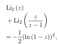
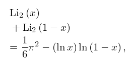
| 25.12.3 | |||
| . | |||
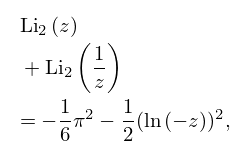
| 25.12.4 | |||
| . | |||
| 25.12.5 | |||
| , . | |||
| 25.12.6 | |||
| . | |||
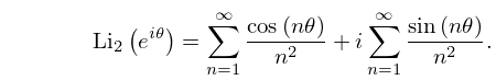
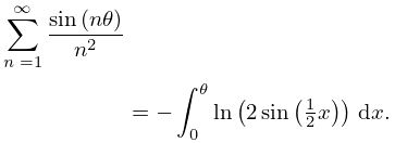
When , , (25.12.1) becomes
| 25.12.7 | |||
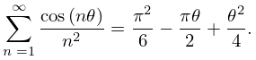
The cosine series in (25.12.7) has the elementary sum
| 25.12.8 | |||
By (25.12.2)
| 25.12.9 | |||
The right-hand side is called Clausen’s integral.
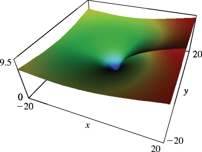
For graphics see Figures 25.12.1 and 25.12.2, and for further properties see Maximon (2003), Kirillov (1995), Lewin (1981), Nielsen (1909), and Zagier (1989).


§25.12(ii) Polylogarithms
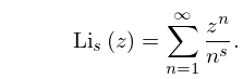
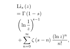
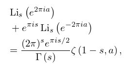
For real or complex and the polylogarithm is defined by
| 25.12.10 | |||
For each fixed complex the series defines an analytic function of for . The series also converges when , provided that . For other values of , is defined by analytic continuation.
The notation was used for in Truesdell (1945) for a series treated in Jonquière (1889), hence the alternative name Jonquière’s function. The special case is the Riemann zeta function: .
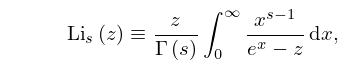
Integral Representation
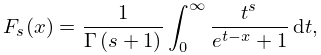
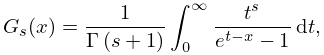
§25.12(iii) Fermi–Dirac and Bose–Einstein Integrals
The Fermi–Dirac and Bose–Einstein integrals are defined by
| 25.12.14 | ||||
| , | ||||
| 25.12.15 | ||||
| , ; or , , | ||||
respectively. Sometimes the factor is omitted. See Cloutman (1989) and Gautschi (1993).
In terms of polylogarithms
| 25.12.16 | ||||
For a uniform asymptotic approximation for see Temme and Olde Daalhuis (1990).
