§18.16 Zeros
Contents
- §18.16(i) Distribution
- §18.16(ii) Jacobi
- §18.16(iii) Ultraspherical, Legendre and Chebyshev
- §18.16(iv) Laguerre
- §18.16(v) Hermite
- §18.16(vi) Additional References
- §18.16(vii) Discriminants
§18.16(i) Distribution
See §18.2(vi).
§18.16(ii) Jacobi
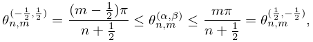
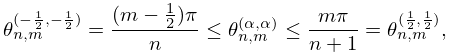
Let , , denote the zeros of as function of with
| 18.16.1 | |||
Then is strictly increasing in and strictly decreasing in ; furthermore, if , then is strictly increasing in .
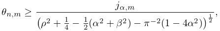
Inequalities
Let be the th positive zero of the Bessel function (§10.21(i)). Then
| 18.16.6 | ||||
| , | ||||
| 18.16.7 | ||||
| , . | ||||
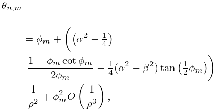
Asymptotic Behavior
Let . Then as , with () and () fixed,
| 18.16.8 | |||
uniformly for , where is an arbitrary constant such that .
Other Bounds
§18.16(iii) Ultraspherical, Legendre and Chebyshev
§18.16(iv) Laguerre
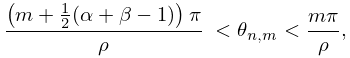
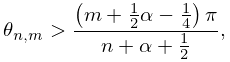
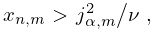
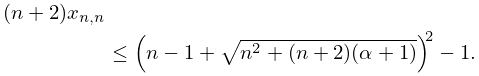
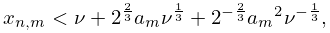
Inequalities
For , and with as in §18.16(ii),
| 18.16.10 | |||
| 18.16.11 | |||
The constant in (18.16.10) is the best possible since the ratio of the two sides of this inequality tends to 1 as .
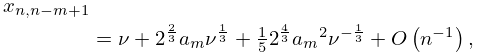
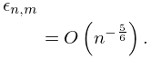
Asymptotic Behavior
§18.16(v) Hermite
All zeros of lie in the open interval . In view of the reflection formula, given in Table 18.6.1, we may consider just the positive zeros , . Arrange them in decreasing order:
| 18.16.16 | |||
Then
| 18.16.17 | |||
where is the th negative zero of (§9.9(i)), , and as with fixed
| 18.16.18 | |||
§18.16(vi) Additional References
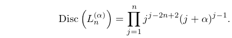
§18.16(vii) Discriminants
The discriminant (18.2.20) can be given explicitly for classical OP’s.
Jacobi
| 18.16.19 | |||
Laguerre
| 18.16.20 | |||
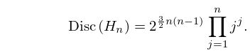
Hermite
| 18.16.21 | |||
