§19.14 Reduction of General Elliptic Integrals
Contents
§19.14(i) Examples
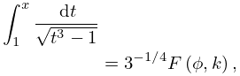
In (19.14.1)–(19.14.3) both the integrand and are assumed to be nonnegative. Cases in which can be included by application of (19.2.10).
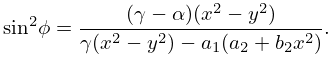
| 19.14.1 | ||||
| , . | ||||
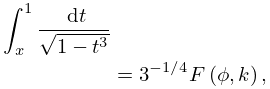
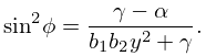
| 19.14.2 | ||||
| , . | ||||
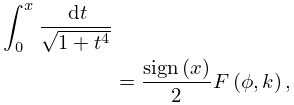
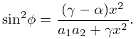
| 19.14.3 | ||||
| , . | ||||
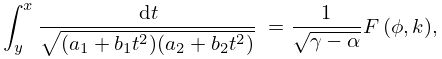
| 19.14.4 | |||
| . | |||
In (19.14.4) , each quadratic polynomial is positive on the interval , and is a permutation of (not all 0 by assumption) such that . More generally in (19.14.4),
| 19.14.5 | |||
where
| 19.14.6 | |||
| 19.14.7 | |||
If , then
| 19.14.8 | |||
If , then
| 19.14.9 | |||
If , then
| 19.14.10 | |||
(These four cases include 12 integrals in Abramowitz and Stegun (1964, p. 596).)
§19.14(ii) General Case
Legendre (1825–1832) showed that every elliptic integral can be expressed in terms of the three integrals in (19.1.2) supplemented by algebraic, logarithmic, and trigonometric functions. The classical method of reducing (19.2.3) to Legendre’s integrals is described in many places, especially Erdélyi et al. (1953b, §13.5), Abramowitz and Stegun (1964, Chapter 17), and Labahn and Mutrie (1997, §3). The last reference gives a clear summary of the various steps involving linear fractional transformations, partial-fraction decomposition, and recurrence relations. It then improves the classical method by first applying Hermite reduction to (19.2.3) to arrive at integrands without multiple poles and uses implicit full partial-fraction decomposition and implicit root finding to minimize computing with algebraic extensions. The choice among 21 transformations for final reduction to Legendre’s normal form depends on inequalities involving the limits of integration and the zeros of the cubic or quartic polynomial. A similar remark applies to the transformations given in Erdélyi et al. (1953b, §13.5) and to the choice among explicit reductions in the extensive table of Byrd and Friedman (1971), in which one limit of integration is assumed to be a branch point of the integrand at which the integral converges. If no such branch point is accessible from the interval of integration (for example, if the integrand is and the interval is [1,2]), then no method using this assumption succeeds.
