§18.39 Applications in the Physical Sciences
Contents
- §18.39(i) Quantum Mechanics
- §18.39(ii) A 3D Separable Quantum System, the Hydrogen Atom
- §18.39(iii) Non Classical Weight Functions of Utility in DVR Method in the Physical Sciences
- §18.39(iv) Coulomb–Pollaczek Polynomials and J-Matrix Methods
- §18.39(v) Other Applications
§18.39(i) Quantum Mechanics
| 18.39.1 | Moved to (errata.1). | ||
| 18.39.2 | Moved to (errata.2). | ||
| 18.39.3 | Moved to (errata.3). | ||
| 18.39.4 | Moved to (errata.4). | ||
| 18.39.5 | Moved to (errata.5). | ||
| 18.39.6 | Moved to (errata.6). | ||
An Introductory Remark
The nature of, and notations and common vocabulary for, the eigenvalues and eigenfunctions of self-adjoint second order differential operators is overviewed in §1.18. This material is employed below with little additional discussion. While non-normalizable continuum, or scattering, states are mentioned, with appropriate references in what follows, focus is on the eigenfunctions corresponding to the point, or discrete, spectrum, and representing bound rather than scattering states, these former being expressed in terms of OP’s or EOP’s.
Introduction and One-Dimensional (1D) Systems
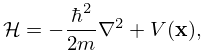
The fundamental quantum Schrödinger operator, also called the Hamiltonian, , is a second order differential operator of the form
| 18.39.7 | |||
| , | |||
where is a spatial coordinate, the mass of the particle with potential energy , is the reduced Planck’s constant, and a finite or infinite interval.
Here the term represents the quantum kinetic energy of a single particle of mass , and its potential energy. As in classical dynamics this sum is the total energy of the one particle system. The properties of determine whether the spectrum, this being the set of eigenvalues of , is discrete, continuous, or mixed, see §1.18. Below we consider two potentials with analytically known eigenfunctions and eigenvalues where the spectrum is entirely point, or discrete, with all eigenfunctions being and forming a complete set. Also presented are the analytic solutions for the , bound state, eigenfunctions and eigenvalues of the Morse oscillator which also has analytically known non-normalizable continuum eigenfunctions, thus providing an example of a mixed spectrum.
However, in the remainder of this section will will assume that the spectrum is discrete, and that the eigenfunctions of form a discrete, normed, and complete basis for a Hilbert space.
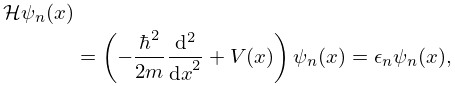
These eigenfunctions are the orthonormal eigenfunctions of the time-independent Schrödinger equation
| 18.39.8 | |||
which in one dimensional systems are typically non-degenerate, namely there is only a single eigenfunction corresponding to each , . The solutions of (18.39.8) are subject to boundary conditions at and . The are the observable energies of the system, and an increasing function of . is referred to as the ground state, all others, in order of increasing energy being excited states. These eigenfunctions are quantum wave-functions whose absolute values squared give the probability density of finding the single particle at hand at position in the th eigenstate, namely that probability is = , being a localized interval on the -axis.
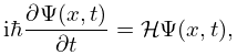
also controls time evolution of the wave function via the time-dependent Schrödinger equation,
| 18.39.9 | |||
where is assumed to be independent of time.
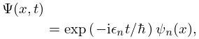
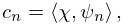
The solutions (18.39.8) are called the stationary states as separation of variables in (18.39.9) yields solutions of form
| 18.39.10 | |||
in which case the probability density is time-independent, as .
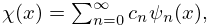
If is an arbitrary unit normalized function in the domain of then, by self-adjointness,
| 18.39.11 | ||||
and
| 18.39.12 | |||
which is the quantum superposition principle. Such a superposition yields continuous time evolution of the probability density .
1D Quantum Systems with Analytically Known Stationary States
Here are three examples of solutions for (18.39.8) for explicit choices of and with the corresponding to the discrete spectrum. All are written in the same form as the product of three factors: the square root of a weight function , the corresponding OP or EOP, and constant factors ensuring unit normalization. Brief mention of non-unit normalized solutions in the case of mixed spectra appear, but as these solutions are not OP’s details appear elsewhere, as referenced.
a) The Harmonic Oscillator
| 18.39.13 | |||
defines the potential for a symmetric restoring force for displacements from . Then is the circular frequency of oscillation (with the ordinary frequency), independent of the amplitude of the oscillations. By Table 18.3.1#12 the normalized stationary states and corresponding eigenvalues are
| 18.39.14 | ||||
| , | ||||
| , | ||||
| 18.39.15 | ||||
Here the are Hermite polynomials, , and . With the normalization factor the are orthonormal in . The spectrum is entirely discrete as in §1.18(v).
b) The Morse Oscillator
| 18.39.16 | |||
allows anharmonic, or amplitude dependent, frequencies of oscillation about , and also escape of the particle to with dissociation energy . The orthonormal stationary states and corresponding eigenvalues are then of the form
| 18.39.17 | ||||
| , | ||||
| , | ||||
and the corresponding eigenvalues are
| 18.39.18 | |||
The functions are expressed in terms of Romanovski–Bessel polynomials, or Laguerre polynomials by (18.34.7_1). The finite system of functions is orthonormal in , see (18.34.7_3). The spectrum is mixed as in §1.18(viii), with the discrete eigenvalues given by (18.39.18) and the continuous eigenvalues by () with corresponding eigenfunctions expressed in terms of Whittaker functions (13.14.3). The corresponding eigenfunction transform is a generalization of the Kontorovich–Lebedev transform §10.43(v), see Faraut (1982, §IV).
c) A Rational SUSY Potential
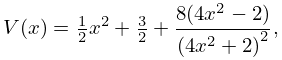
The Schrödinger equation with potential
| 18.39.19 | |||
and , has eigenfunctions
| 18.39.20 | |||
| , | |||
and eigenvalues , with as above, with the weight function of (18.36.10), and a type III Hermite EOP defined by (18.36.8) and (18.36.9). There is no need for a normalization constant here, as appropriate constants already appear in §18.36(vi). The spectrum is entirely discrete as in §1.18(v).
An important, and perhaps unexpected, feature of the EOP’s is now pointed out by noting that for 1D Schrödinger operators, or equivalent Sturm-Liouville ODEs, having discrete spectra with eigenfunctions vanishing at the end points, in this case see Simon (2005c, Theorem 3.3, p. 35), such eigenfunctions satisfy the Sturm oscillation theorem. Namely the th eigenfunction, listed in order of increasing eigenvalues, starting at , has precisely nodes, as real zeros of wave-functions away from boundaries are often referred to. This seems odd at first glance as is a polynomial of order for , seemingly suggesting that for , this being the first excited state, i.e., , there might be 3 nodes, rather than Sturm’s 1. This is illustrated in Figure 18.39.1 where the first and fourth excited state eigenfunctions of the Schrödinger operator with the rationally extended harmonic potential, of (18.39.19), are shown, and compared with the first and fourth excited states of the harmonic oscillator eigenfunctions of (18.39.14) of paragraph a), above. Both satisfy Sturm’s theorem. Thus the two missing quantum numbers corresponding to EOP’s of order and of the type III Hermite EOP’s are offset in the node counts by the fact that all excited state eigenfunctions also have two missing real zeros. Kuijlaars and Milson (2015, §1) refer to these, in this case complex zeros, as exceptional, as opposed to regular, zeros of the EOP’s, these latter belonging to the (real) orthogonality integration range.

Other Analytically Solved Schrödinger Equations
These are overviewed in §18.38(iii), and §18.36(vi), and typically involve OP’s or EOP’s.
§18.39(ii) A 3D Separable Quantum System, the Hydrogen Atom
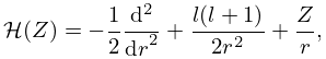
Analogous to (18.39.7) the 3D Schrödinger operator is
| 18.39.21 | |||
| , | |||
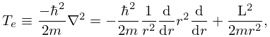
where is the Laplacian (1.5.17). Now use spherical coordinates (1.5.16) with instead of , and assume the potential to be radial. Then write instead of . By (1.5.17) the first term in (18.39.21), which is the quantum kinetic energy operator , can be written in spherical coordinates as
| 18.39.22 | |||
where is the (squared) angular momentum operator (14.30.12). The eigenfunctions of are the spherical harmonics with eigenvalues , each with degeneracy as . See (14.30.11).
Analogous to (18.39.8) the 3D time-independent Schrödinger equation with potential is
| 18.39.23 | |||
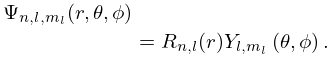
Since the operators and commute and have simultaneous eigenfunctions (see §1.3(iv)), the wave function separates as
| 18.39.24 | |||
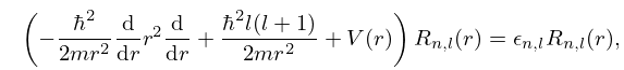
Orthogonality and normalization of eigenfunctions of this form is respect to the measure . Substitution of (18.39.24) into (18.39.23) then gives the ordinary differential equation for the radial wave function ,
| 18.39.25 | |||
| . | |||
The eigenvalues and radial wave functions are independent of and they both do depend on due to the presence of the ‘fictitious’ centrifugal potential , which is a result of the choice of co-ordinate system, and not the physical potential energy of interaction .
An alternative, and often used, form of (18.39.25) is that for the spherical radial function ,
| 18.39.26 | |||
where the orthogonality measure is now ,
The Quantum Coulomb Problem
In the case of a single electron, charge and mass , interacting with a fixed (infinite mass) nucleus of charge at the co-ordinate origin, with the choice of SI units, . This is Coulomb’s Law. The spectrum is mixed, as in §1.18(viii), the positive energy, non-, scattering states are the subject of Chapter 33.
The non-relativistic Schrödinger equation describing a single, bound (negative energy) electron, in an eigenstate of energy is:
| 18.39.27 | |||
In what follows the radial and spherical radial eigenfunctions corresponding to (18.39.27) are found in four different notations, with identical eigenvalues, all of which appear in the current and past mathematical and theoretical physics and chemistry literatures, regarding this central problem. Explicit normalization is given for the second, third, and fourth of these, paragraphs c) and d), below. All results are presented in Hartree atomic units, or a.u., i.e., , Mohr and Taylor (2005, Table XXX, p. 71), where the relationship of to SI units is spelled out.
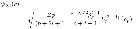
a) Spherical Radial Coulomb Wave Functions Expressed in terms of Laguerre OP’s
The functions satisfy the equation,
| 18.39.28 | |||
with an infinite set of orthonormal eigenfunctions
| 18.39.29 | |||
| ; , | |||
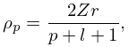
here being the order of the Laguerre polynomial, of Table 18.8.1, line 11, and the angular momentum quantum number, and where
| 18.39.30 | |||
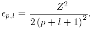
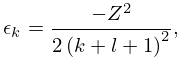
with eigenvalues
| 18.39.31 | |||
See Titchmarsh (1962a, pp. 99–100).
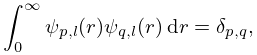
Orthogonality, with measure for , for fixed
| 18.39.32 | |||
noting that the are real, follows from the fact that the Schrödinger operator of (18.39.28) is self-adjoint, or from the direct derivation of Dunkl (2003). This is not the orthogonality of Table 18.8.1, as the co-ordinate arguments depend, independently on and . This indicates that the Laguerre polynomials appearing in (18.39.29) are not classical OP’s, and in fact, even though infinite in number for fixed , do not form a complete set. Namely for fixed the infinite set labeled by describe only the bound states for that single , omitting the continuum briefly mentioned below, and which is the subject of Chapter 33, and so an unusual example of the mixed spectra of §1.18(viii).
b) The Bohr Quantum Number
The fact that both the eigenvalues of (18.39.31) and the scaling of the co-ordinate in the eigenfunctions, (18.39.30), depend on the sum leads to the substitution
| 18.39.33 | |||
where is now the Bohr Principle Quantum Number.
Physical scientists use the of Bohr as, to th and st order, it describes the structure and organization of the Periodic Table of the Chemical Elements of which the Hydrogen atom is only the first.
This follows from the fact that the eigenvalues (18.39.31), depend only on the single quantum number , the Bohr Principal quantum number, , and depend explicitly neither on nor . Thus the overall degeneracy of the solutions (18.39.29) (the number of independent eigenfunctions corresponding to a single eigenvalue (18.39.31) for all values of and ) consistent with each is , which controls the lengths of the rows in the Periodic Table. Interactions between electrons, in many electron atoms, breaks this degeneracy as a function of , but still dominates.
c) Spherical Radial Coulomb Wave Functions
The solution, (18.39.29), of the spherical radial equation (18.39.28), now expressed in terms of the Bohr quantum number , is
| 18.39.34 | |||
| , | |||
| 18.39.35 | |||
thus recapitulating, for , line 11 of Table 18.8.1, now shown with explicit normalization for the measure . This is also the normalization and notation of Chapter 33 for , and the notation of Weinberg (2013, Chapter 2). The radial Coulomb wave functions , solutions of
| 18.39.36 | |||
with and being those of (18.39.35), are then
| 18.39.37 | |||
normalized with measure , .
d) Radial Coulomb Wave Functions Expressed in Terms of the Associated Coulomb–Laguerre OP’s
The same solutions as in paragraph c), above, appear frequently in the literature in terms of associated Laguerre polynomials, which are referred to here as associated Coulomb–Laguerre polynomials to avoid confusion with the more recent meaning of ‘associated’ of §18.30. The associated Coulomb–Laguerre polynomials are defined as
| 18.39.38 | |||
where
| 18.39.39 | |||
see Bethe and Salpeter (1957, p. 13), Pauling and Wilson (1985, pp. 130, 131); and noting that this differs from the Rodrigues formula of (18.5.5) for the Laguerre OP’s, in the omission of an in the denominator.
From (18.9.23) and (18.5.5) with Table 18.5.1, line 8:
| 18.39.40 | |||
and thus replacing by as in Table 18.8.1, line 11, or as in (18.39.33),
| 18.39.41 | |||
(where the minus sign is often omitted, as it arises as an arbitrary phase when taking the square root of the real, positive, norm of the wave function), allowing equation (18.39.37) to be rewritten in terms of the associated Coulomb–Laguerre polynomials .
| 18.39.42 | |||
Derivations of (18.39.42) appear in Bethe and Salpeter (1957, pp. 12–20), and Pauling and Wilson (1985, Chapter V and Appendix VII), where the derivations are based on (18.39.36), and is also the notation of Piela (2014, §4.7), typifying the common use of the associated Coulomb–Laguerre polynomials in theoretical quantum chemistry. In all of these references these OP’s are simply referred to as the associated Laguerre OP’s.
The Relativistic Quantum Coulomb Problem
Bound state solutions to the relativistic Dirac Equation, for this same problem of a single electron attracted by a nucleus with protons, involve Laguerre polynomials of fractional index. A relativistic treatment becoming necessary as becomes large as corrections to the non-relativistic Schrödinger picture are of approximate order , being the dimensionless fine structure constant , where is the speed of light. See Martinez-y-Romero (2000).
The Quantum Coulomb Problem: Scattering States
The positive energy (scattering) eigenfunctions for the above Coulomb problem, with potential are discussed in Chapter 33 for each integer . These, taken together with the infinite sets of bound states for each , form complete sets. As the scattering eigenfunctions of Chapter 33, are not OP’s, their further discussion is deferred to §18.39(iv), where discretized representations of these scattering states are introduced, Laguerre and Pollaczek OP’s then playing a key role.
§18.39(iii) Non Classical Weight Functions of Utility in DVR Method in the Physical Sciences
Shizgal (2015) gives a broad overview of techniques and applications of spectral and pseudo-spectral methods to problems arising in theoretical chemistry, chemical kinetics, transport theory, and astrophysics.
The discrete variable representations (DVR) analysis is simplest when based on the classical OP’s with their analytically known recursion coefficients (Table 3.5.17_5), or those non-classical OP’s which have analytically known recursion coefficients, making stable computation of the and , from the J-matrix as in §3.5(vi), straightforward. For many applications the natural weight functions are non-classical, and thus the OP’s and the determination of the Gaussian quadrature points and weights represent a computational challenge. Table 18.39.1 lists typical non-classical weight functions, many related to the non-classical Freud weights of §18.32, and §32.15, all of which require numerical computation of the recursion coefficients (i.e., the J-matrix elements) as in Gautschi (1968), Golub and Welsch (1969), Gordon (1968). A major difficulty in such calculations, loss of precision, is addressed in Gautschi (2009) where use of variable precision arithmetic is discussed and employed. Shizgal (2015, Chapter 2), contains a broad-ranged discussion of methods and applications for these, and other, non-classical weight functions. Further details of such calculations are contained in the papers cited.
| Name of OP System | Notation | Applications | ||
|---|---|---|---|---|
| Freud-Bimodal | Fokker–Planck DVRb,c | |||
| Quartic Freud | §32.15 and application refs. therein: Quantum Gravity and Graph Theory Combinatorics | |||
| Half-Freud Druvesteyn | Electron Transport in Plasmasd | |||
| Half-Freud Gaussian | Fokker–Planck DVRe | |||
| Half-Freud Maxwell | Kinetic Theoryf,g and Fokker–Planck DVRsh | |||
| Half-Rys | Quantum Chemistry Quadraturesi,j | |||
| Multi-Exponential | Quadrature Sums of Exponentialsk | |||
| Radiative Transfer | Radiative Transferl |
a) Shizgal (2015), b) Blackmore et al. (1986), c) Gammaitoni et al. (1998), d) Liboff (2003). e) Garashchuk and Light (2001), f) Gross and Ziering (1958), g) Desai and Nelkin (1966), h) Blackmore and Shizgal (1985), i) Helgaker et al. (2012), j) Rys et al. (1983), k) Gill and Chen (2003), l) Gander and Karp (2001).
§18.39(iv) Coulomb–Pollaczek Polynomials and J-Matrix Methods
The bound state eigenfunctions of the radial Coulomb Schrödinger operator are discussed in §§18.39(i) and 18.39(ii), and the -function normalized (non-) in Chapter 33, where the solutions appear as Whittaker functions. These same solutions are expressed here in terms of Laguerre and Pollaczek OP’s. The technique to accomplish this follows the DVR idea, in which methods are based on finding tridiagonal representations of the co-ordinate, . Here tridiagonal representations of simple Schrödinger operators play a similar role. The radial operator (18.39.28)
| 18.39.43 | |||
| , | |||
is tridiagonalized in the complete non-orthogonal (with measure , ) basis of Laguerre functions:
| 18.39.44 | |||
| , | |||
where is a real, positive, scaling factor, and a non-negative integer.
As in this subsection both positive (repulsive) and negative (attractive) Coulomb interactions are discussed, the prefactor of in (18.39.43) has been set to , rather than the of (18.39.28) implying that is an attractive interaction, being repulsive.
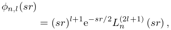
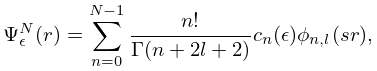
This operator may be discretized by projecting it onto the sub-space defined by the first members, , of the complete basis of (18.39.44), the eigenfunctions, may be expressed as
| 18.39.45 | |||
with matrix eigenvalues , , and the eigenvectors, , are determined by the recursion relation (18.39.46) below.
Following the method of Schwartz (1961), Yamani and Reinhardt (1975), Bank and Ismail (1985), and Ismail (2009, §5.8) have shown this is equivalent to determination of such that in the recursion scheme
| 18.39.46 | |||
with initial data , , where
| 18.39.47 | |||
and
| 18.39.48 | |||
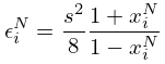
which maps onto . The recursion of (18.39.46) is that for the type 2 Pollaczek polynomials of (18.35.2), with , , and , and terminates for being a zero of the polynomial of order . Thus the and the eigenvalues
| 18.39.49 | |||
are determined by the zeros, of the Pollaczek polynomial .
The Coulomb–Pollaczek Polynomials
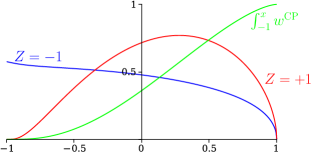
The polynomials , for both positive and negative , define the Coulomb–Pollaczek polynomials (CP OP’s in what follows), see Yamani and Reinhardt (1975, Appendix B, and §IV). For these are the repulsive CP OP’s with corresponding to the continuous spectrum of , , and for we have the attractive CP OP’s, where the spectrum is complemented by the infinite set of bound state eigenvalues for fixed . These cases correspond to the two distinct orthogonality conditions of (18.35.6) and (18.35.6_3).
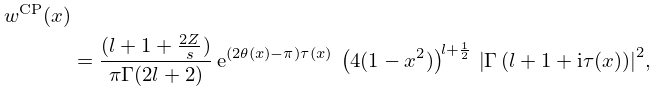
Given that in both the attractive and repulsive cases, the expression for the absolutely continuous, , part of the function of (18.35.6) may be simplified:
| 18.39.50 | |||
| , . | |||
Note that violation of the Favard inequality, possible when , results in a zero or negative weight function. While in the basis of (18.39.44) is simply a variational parameter, care must be taken, or the relationship between the results of the matrix variational approximation and the Pollaczek polynomials is lost, although this has no effect on the use of the variational approximations Reinhardt (2021a, b). Graphs of the weight functions of (18.39.50) are shown in Figure 18.39.2.
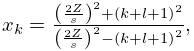
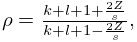
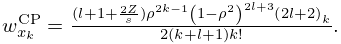
In the attractive case (18.35.6_4) for the discrete parts of the weight function where with , are also simplified:
| 18.39.51 | ||||
The weight functions for both the attractive and repulsive cases are now unit normalized, see Bank and Ismail (1985), and Ismail (2009). Note that these discrete , from (18.39.51), giving, for , ,
| 18.39.52 | |||
| , | |||
which is Bohr’s quantization for the Coulomb bound state energies (18.39.31). The Schrödinger operator essential singularity, seen in the accumulation of discrete eigenvalues for the attractive Coulomb problem, is mirrored in the accumulation of jumps in the discrete Pollaczek–Stieltjes measure as . As the Coulomb–Pollaczek OP’s are members of the Nevai-Blumenthal class, this is, for , a physical example of the properties of the zeros of such OP’s, and their possible accumulation at , as discussed in §18.2(xi).
Discretized and Continuum Expansions of Scattering Eigenfunctions in terms of Pollaczek Polynomials: J-matrix Theory
The Coulomb–Pollaczek polynomials provide alternate representations of the positive energy Coulomb wave functions of Chapter 33. For either sign of , and chosen such that , , truncation of the basis to terms, with , the discrete eigenvectors are the orthonormal functions
| 18.39.53 | |||
| . | |||
With the functions normalized as with measure are, formally,
| 18.39.54 | |||
| , | |||
which corresponds to the exact results, in terms of Whittaker functions, of §§33.2 and 33.14, in the sense that projections onto the functions , the functions bi-orthogonal to , are identical. Full expressions for both and are given in Yamani and Reinhardt (1975) and it is seen that = where is the Gaussian-Pollaczek quadrature weight at , and is the Gaussian-Pollaczek weight function at the same quadrature abscissa. This equivalent quadrature relationship, see Heller et al. (1973), Yamani and Reinhardt (1975), allows extraction of scattering information from the finite dimensional functions of (18.39.53), provided that such information involves potentials, or projections onto functions, exactly expressed, or well approximated, in the finite basis of (18.39.44). The equivalent quadrature weight, , also forms the foundation of a novel inversion of the Stieltjes–Perron moment inversion discussed in §18.40(ii).
The fact that non- continuum scattering eigenstates may be expressed in terms or (infinite) sums of functions allows a reformulation of scattering theory in atomic physics wherein no non- functions need appear. As this follows from the three term recursion of (18.39.46) it is referred to as the J-Matrix approach, see (3.5.31), to single and multi-channel scattering numerics. See Yamani and Fishman (1975) for for expansions of both the regular and irregular spherical Bessel functions, which are the Pollaczeks with , and Coulomb functions for fixed , Broad and Reinhardt (1976) for a many particle example, and the overview of Alhaidari et al. (2008). Mathematical underpinnings appear in Ismail (2009, §5.8), and Ismail and Koelink (2011).
§18.39(v) Other Applications
For applications of Legendre polynomials in fluid dynamics to study the flow around the outside of a puff of hot gas rising through the air, see Paterson (1983). For applications and an extension of the Szegő–Szász inequality (18.14.20) for Legendre polynomials () to obtain global bounds on the variation of the phase of an elastic scattering amplitude, see Cornille and Martin (1972, 1974). For physical applications of -Laguerre polynomials see §17.17. For interpretations of zeros of classical OP’s as equilibrium positions of charges in electrostatic problems (assuming logarithmic interaction), see Ismail (2000a, b).
