§10.21 Zeros
Contents
- §10.21(i) Distribution
- §10.21(ii) Analytic Properties
- §10.21(iii) Infinite Products
- §10.21(iv) Monotonicity Properties
- §10.21(v) Inequalities
- §10.21(vi) McMahon’s Asymptotic Expansions for Large Zeros
- §10.21(vii) Asymptotic Expansions for Large Order
- §10.21(viii) Uniform Asymptotic Approximations for Large Order
- §10.21(ix) Complex Zeros
- §10.21(x) Cross-Products
- §10.21(xi) Riccati–Bessel Functions
- §10.21(xii) Zeros of
- §10.21(xiii) Rayleigh Function
- §10.21(xiv) -Zeros
§10.21(i) Distribution
The zeros of any cylinder function or its derivative are simple, with the possible exceptions of in the case of the functions, and in the case of the derivatives.
If is real, then , , , and , each have an infinite number of positive real zeros. All of these zeros are simple, provided that in the case of , and in the case of . When all of their zeros are simple, the th positive zeros of these functions are denoted by , , , and respectively, except that is counted as the first zero of . Since we have
| 10.21.1 | ||||
| . | ||||
When , the zeros interlace according to the inequalities
| 10.21.2 | ||||
| 10.21.3 | |||
For an extension see Pálmai and Apagyi (2011).
The positive zeros of any two real distinct cylinder functions of the same order are interlaced, as are the positive zeros of any real cylinder function and the contiguous function . See also Elbert and Laforgia (1994).
When the zeros of are all real. If and is not an integer, then the number of complex zeros of is . If is odd, then two of these zeros lie on the imaginary axis.
If , then the zeros of are all real.
For information on the real double zeros of and when and , respectively, see Döring (1971) and Kerimov and Skorokhodov (1986). The latter reference also has information on double zeros of the second and third derivatives of and .
No two of the functions , , , have any common zeros other than ; see Watson (1944, §15.28).
§10.21(ii) Analytic Properties
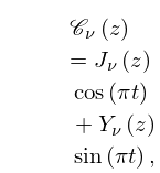
If is a zero of the cylinder function
| 10.21.4 | |||
where is a parameter, then
| 10.21.5 | |||
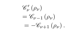
If is a zero of , then
| 10.21.6 | |||
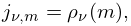
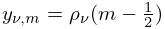
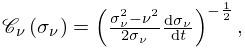
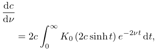
The parameter may be regarded as a continuous variable and , as functions , of . If and these functions are fixed by
| 10.21.7 | ||||
then
| 10.21.8 | ||||
| , | ||||
| , | ||||
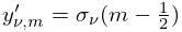
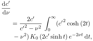
| 10.21.9 | ||||
| , | ||||
| . | ||||
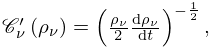
| 10.21.10 | ||||
| 10.21.11 | |||
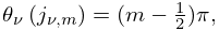
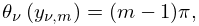
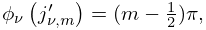
The functions and are related to the inverses of the phase functions and defined in §10.18(i): if , then
| 10.21.12 | ||||
| , | ||||
| 10.21.13 | ||||
| . | ||||
For sign properties of the forward differences that are defined by
| 10.21.14 | ||||
when , and similarly for , see Lorch and Szegő (1963, 1964), Lorch et al. (1970, 1972), and Muldoon (1977).
Some information on the distribution of and for real values of and is given in Muldoon and Spigler (1984).
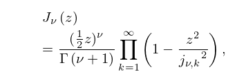
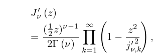
§10.21(iii) Infinite Products
| 10.21.15 | ||||
| , | ||||
| 10.21.16 | ||||
| . | ||||
§10.21(iv) Monotonicity Properties
Any positive zero of the cylinder function and any positive zero of such that are definable as continuous and increasing functions of :
| 10.21.17 | |||
| 10.21.18 | |||
where is defined in §10.25(ii).
In particular, , , , and are increasing functions of when . It is also true that the positive zeros and of and , respectively, are increasing functions of when , provided that in the latter case when .
and are decreasing functions of when for .
§10.21(v) Inequalities
For bounds for the smallest real or purely imaginary zeros of when is real see Ismail and Muldoon (1995).
§10.21(vi) McMahon’s Asymptotic Expansions for Large Zeros
If is fixed, , and , then
| 10.21.19 | |||
where for , for . With , the right-hand side is the asymptotic expansion of for large .
| 10.21.20 | |||
where for , for , and for .
For the next three terms in (10.21.19) and the next two terms in (10.21.20) see Bickley et al. (1952, p. xxxvii) or Olver (1960, pp. xvii–xviii).
For error bounds see Wong and Lang (1990), Wong (1995), and Elbert and Laforgia (2000). See also Laforgia (1979).
For the th positive zero of Wong and Lang (1990) gives the corresponding expansion
| 10.21.21 | |||
where if , and if . An error bound is included for the case .
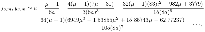
§10.21(vii) Asymptotic Expansions for Large Order
Let , , and be defined as in §10.21(ii) and , , , and denote the modulus and phase functions for the Airy functions and their derivatives as in §9.8.
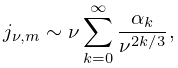
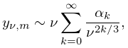
As with fixed,
| 10.21.22 | |||
| 10.21.23 | |||
where is given by
| 10.21.24 | |||
and
| 10.21.25 | ||||
| 10.21.26 | ||||
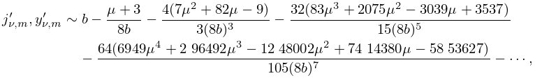
As with fixed,
| 10.21.27 | |||
| 10.21.28 | |||
where is given by
| 10.21.29 | |||
and
| 10.21.30 | ||||
| 10.21.31 | ||||
In particular, with the notation as below,
| 10.21.32 | |||
| 10.21.33 | |||
| 10.21.34 | |||
| 10.21.35 | |||
and
| 10.21.36 | |||
| 10.21.37 | |||
| 10.21.38 | |||
| 10.21.39 | |||
Here , , , are the th negative zeros of , , , , respectively (§9.9), , , , are given by (10.21.25), (10.21.26), (10.21.30), and (10.21.31), with in the case of and , in the case of and , in the case of and , in the case of and .
For error bounds for (10.21.32) see Qu and Wong (1999); for (10.21.36) and (10.21.37) see Elbert and Laforgia (1997). See also Spigler (1980).
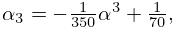
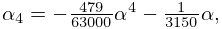
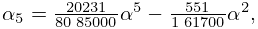
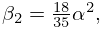
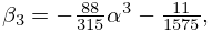
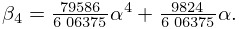
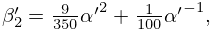
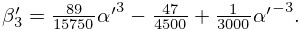
For the first zeros rounded numerical values of the coefficients are given by
| 10.21.40 | ||||
For numerical coefficients for see Olver (1951, Tables 3–6).
The expansions (10.21.32)–(10.21.39) become progressively weaker as increases. The approximations that follow in §10.21(viii) do not suffer from this drawback.
§10.21(viii) Uniform Asymptotic Approximations for Large Order
As the following four approximations hold uniformly for :
| 10.21.41 | |||
| , | |||
| 10.21.42 | |||
| , | |||
| 10.21.43 | |||
| , | |||
| 10.21.44 | |||
| . | |||
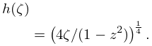
Here and denote respectively the zeros of the Airy function and its derivative ; see §9.9. Next, is the inverse of the function defined by (10.20.3). and are defined by (10.20.11) and (10.20.12) with . Lastly,
| 10.21.45 | |||
(Note: If the term in (10.21.43) is omitted, then the uniform character of the error term is destroyed.)
§10.21(ix) Complex Zeros
This subsection describes the distribution in of the zeros of the principal branches of the Bessel functions of the second and third kinds, and their derivatives, in the case when the order is a positive integer . For further information, including uniform asymptotic expansions, extensions to other branches of the functions and their derivatives, and extensions to half-integer values of the order, see Olver (1954). (There is an inaccuracy in Figures 11 and 14 in this reference. Each curve that represents an infinite string of nonreal zeros should be located on the opposite side of its straight line asymptote. This inaccuracy was repeated in Abramowitz and Stegun (1964, Figures 9.5 and 9.6). See Kerimov and Skorokhodov (1985a, b) and Figures 10.21.3–10.21.6.)
See also Cruz and Sesma (1982), Cruz et al. (1991), Kerimov and Skorokhodov (1984c, 1987, 1988), Kokologiannaki et al. (1992), and references supplied in §10.75(iii). For describing the distribution of complex zeros by methods based on the Liouville–Green (WKB) approximation for linear homogeneous second-order differential equations, see Segura (2013).
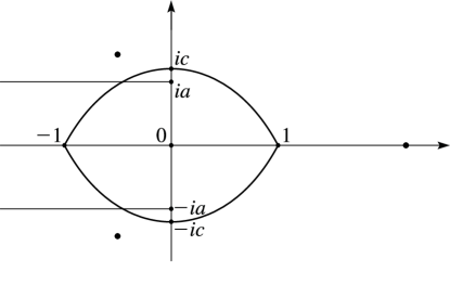
Zeros of and
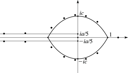
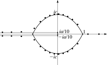
In Figures 10.21.1, 10.21.3, and 10.21.5 the two continuous curves that join the points are the boundaries of , that is, the eye-shaped domain depicted in Figure 10.20.3. These curves therefore intersect the imaginary axis at the points , where .
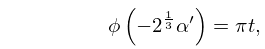
The first set of zeros of the principal value of are the points , , on the positive real axis (§10.21(i)). Secondly, there is a conjugate pair of infinite strings of zeros with asymptotes , where
| 10.21.46 | |||
Lastly, there are two conjugate sets, with zeros in each set, that are asymptotically close to the boundary of as . Figures 10.21.1, 10.21.3, and 10.21.5 plot the actual zeros for , and , respectively.
The zeros of have a similar pattern to those of .
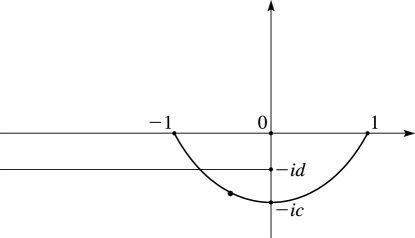


Zeros of , , ,
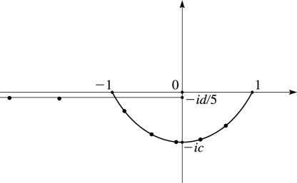
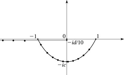
In Figures 10.21.2, 10.21.4, and 10.21.6 the continuous curve that joins the points is the lower boundary of .
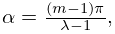
The first set of zeros of the principal value of is an infinite string with asymptote , where
| 10.21.47 | |||
The only other set comprises zeros that are asymptotically close to the lower boundary of as . Figures 10.21.2, 10.21.4, and 10.21.6 plot the actual zeros for , and , respectively.
The zeros of have a similar pattern to those of . The zeros of and are the complex conjugates of the zeros of and , respectively.
Zeros of and
§10.21(x) Cross-Products
Throughout this subsection we assume , , , and we denote by .
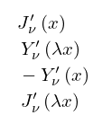
The zeros of the functions
| 10.21.48 | |||
and
| 10.21.49 | |||
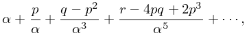
are simple and the asymptotic expansion of the th positive zero as is given by
| 10.21.50 | |||
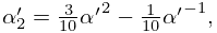
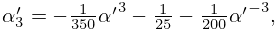
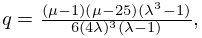
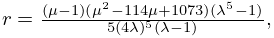
where, in the case of (10.21.48),
| 10.21.51 | ||||
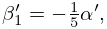
and, in the case of (10.21.49),
| 10.21.52 | ||||
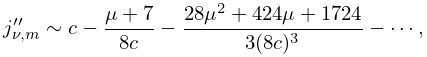
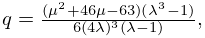
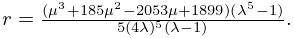
The asymptotic expansion of the large positive zeros (not necessarily the th) of the function
| 10.21.53 | |||
is given by (10.21.50), where
| 10.21.54 | ||||
Higher coefficients in the asymptotic expansions in this subsection can be obtained by expressing the cross-products in terms of the modulus and phase functions (§10.18), and then reverting the asymptotic expansion for the difference of the phase functions.
§10.21(xi) Riccati–Bessel Functions
The Riccati–Bessel functions are and . Except possibly for their zeros are the same as those of and , respectively. For information on the zeros of the derivatives of Riccati–Bessel functions, and also on zeros of their cross-products, see Boyer (1969). This information includes asymptotic approximations analogous to those given in §§10.21(vi), 10.21(vii), and 10.21(x).
§10.21(xii) Zeros of
For properties of the positive zeros of the function , with and real, see Landau (1999).
