§10.43 Integrals
Contents
- §10.43(i) Indefinite Integrals
- §10.43(ii) Integrals over the Intervals and
- §10.43(iii) Fractional Integrals
- §10.43(iv) Integrals over the Interval ()
- §10.43(v) Kontorovich–Lebedev Transform
- §10.43(vi) Compendia
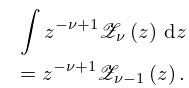
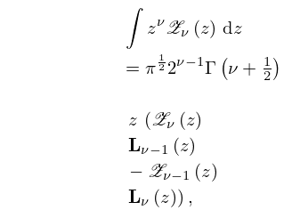
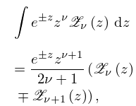
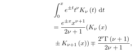
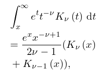
§10.43(i) Indefinite Integrals
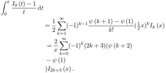
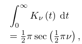
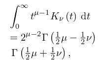
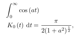
§10.43(ii) Integrals over the Intervals and
| 10.43.4 | |||
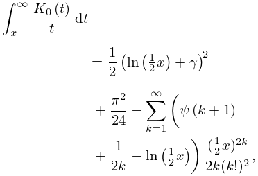
| 10.43.5 | |||
where and is Euler’s constant (§5.2).
| 10.43.6 | |||
| . | |||
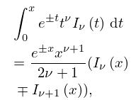
| 10.43.7 | |||
| , | |||
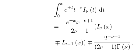
| 10.43.8 | |||
| . | |||
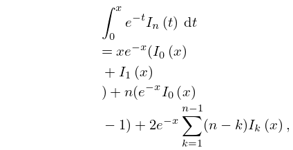
| 10.43.9 | |||
| , | |||
| 10.43.10 | |||
| . | |||
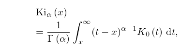
§10.43(iii) Fractional Integrals
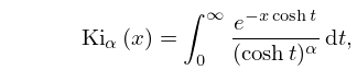
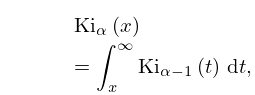
The Bickley function is defined by
| 10.43.11 | |||
when and , and by analytic continuation elsewhere. Equivalently,
| 10.43.12 | |||
| . | |||
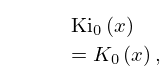
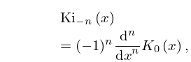
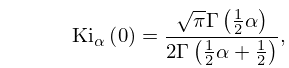
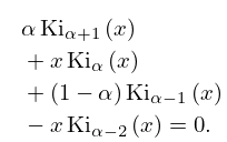
Properties
| 10.43.13 | |||
| 10.43.14 | |||
| 10.43.15 | |||
| . | |||
| 10.43.16 | |||
| . | |||
| 10.43.17 | |||
§10.43(iv) Integrals over the Interval ()
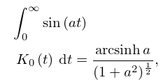
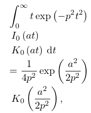
| 10.43.18 | |||
| . | |||
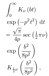
| 10.43.19 | |||
| . | |||
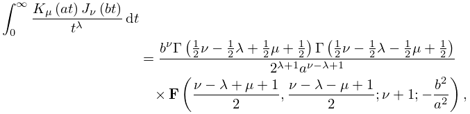
| 10.43.20 | ||||
| , | ||||
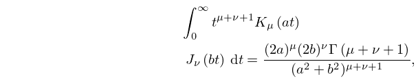
| 10.43.21 | ||||
| . | ||||
When ,
| 10.43.22 | |||
For the second equation there is a cut in the -plane along the interval , and all quantities assume their principal values (§4.2(i)). For the Ferrers function and the associated Legendre function , see §§14.3(i) and 14.21(i).
| 10.43.23 | ||||
| , | ||||
| 10.43.24 | ||||
| , , | ||||
| 10.43.25 | ||||
| , . | ||||
| 10.43.26 | ||||
| . | ||||
For the hypergeometric function see §15.2(i).
| 10.43.27 | ||||
| . | ||||
| 10.43.28 | ||||
| , | ||||
| 10.43.29 | ||||
| . | ||||
§10.43(v) Kontorovich–Lebedev Transform
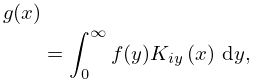
The Kontorovich–Lebedev transform of a function is defined as
| 10.43.30 | |||
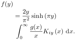
Then
| 10.43.31 | |||
provided that either of the following sets of conditions is satisfied:
-
(a)
On the interval , is continuously differentiable and each of and is absolutely integrable.
-
(b)
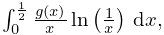
is piecewise continuous and of bounded variation on every compact interval in , and each of the following integrals
| 10.43.32 | |||
-
converges.
§10.43(vi) Compendia
For collections of integrals of the functions and , including integrals with respect to the order, see Apelblat (1983, §12), Erdélyi et al. (1953b, §§7.7.1–7.7.7 and 7.14–7.14.2), Erdélyi et al. (1954a, b), Gradshteyn and Ryzhik (2000, §§5.5, 6.5–6.7), Gröbner and Hofreiter (1950, pp. 197–203), Luke (1962), Magnus et al. (1966, §3.8), Marichev (1983, pp. 191–216), Oberhettinger (1972), Oberhettinger (1974, §§1.11 and 2.7), Oberhettinger (1990, §§1.17–1.20 and 2.17–2.20), Oberhettinger and Badii (1973, §§1.15 and 2.13), Okui (1974, 1975), Prudnikov et al. (1986b, §§1.11–1.12, 2.15–2.16, 3.2.8–3.2.10, and 3.4.1), Prudnikov et al. (1992a, §§3.15, 3.16), Prudnikov et al. (1992b, §§3.15, 3.16), Watson (1944, Chapter 13), and Wheelon (1968).
