.pptv世界杯相声汇_『网址:68707.vip』世界杯决赛乌龙球_b5p6v3_2022年11月30日4时58分48秒_ucgsamhsa

(0.003 seconds)

21—30 of 155 matching pages

21: Bibliography Y

… ►

A. I. Yablonskiĭ (1959) On rational solutions of the second Painlevé equation. Vesti Akad. Navuk. BSSR Ser. Fiz. Tkh. Nauk. 3, pp. 30–35 (Russian).

ⓘ

Referenced by:: §32.8(ii).
Encodings:: BibTeX

… ►

H. A. Yamani and W. P. Reinhardt (1975)

L

-squared discretizations of the continuum: Radial kinetic energy and the Coulomb Hamiltonian. Phys. Rev. A 11 (4), pp. 1144–1156.

ⓘ

Referenced by:: §18.39(iv), §18.39(iv), §18.39(iv), §18.40(ii).
Encodings:: BibTeX

…

22: Bibliography N

… ►

A. Natarajan and N. Mohankumar (1993) On the numerical evaluation of the generalised Fermi-Dirac integrals. Comput. Phys. Comm. 76 (1), pp. 48–50.

ⓘ

External Links:: ISSN 0010-4655, Document, ZentralBlatt
Referenced by:: §25.18(i).
Encodings:: BibTeX

… ►

E. Neuman (1969a) Elliptic integrals of the second and third kinds. Zastos. Mat. 11, pp. 99–102.

ⓘ

Notes:: Includes Algol program.
External Links:: MathReview
Referenced by:: §19.39(iii).
Encodings:: BibTeX

►

E. Neuman (1969b) On the calculation of elliptic integrals of the second and third kinds. Zastos. Mat. 11, pp. 91–94.

ⓘ

External Links:: MathReview, ZentralBlatt
Referenced by:: §19.36(ii).
Encodings:: BibTeX

… ►

P. Nevai (1986) Géza Freud, orthogonal polynomials and Christoffel functions. A case study. J. Approx. Theory 48 (1), pp. 3–167.

ⓘ

External Links:: ISSN 0021-9045, Document, MathReview (T. S. Chihara), ZentralBlatt
Referenced by:: §18.32.
Encodings:: BibTeX

… ►

V. Yu. Novokshënov (1985) The asymptotic behavior of the general real solution of the third Painlevé equation. Dokl. Akad. Nauk SSSR 283 (5), pp. 1161–1165 (Russian).

ⓘ

Notes:: In Russian. English translation: Sov. Math., Dokl. 30(1988), no. 8, pp. 666–668.
External Links:: ISSN 0002-3264, MathReview (Vojislav Marić), ZentralBlatt
Referenced by:: §32.11(iv).
Encodings:: BibTeX

…

23: Bibliography L

… ►

D. Le (1985) An efficient derivative-free method for solving nonlinear equations. ACM Trans. Math. Software 11 (3), pp. 250–262.

ⓘ

Notes:: Corrigendum, ibid. 15(3) (1989), 287
External Links:: ISSN 0098-3500, Document, MathReview (T. Feagin), ZentralBlatt
Referenced by:: §3.8(iii).
Encodings:: BibTeX

… ►

A. Leitner and J. Meixner (1960) Eine Verallgemeinerung der Sphäroidfunktionen. Arch. Math. 11, pp. 29–39.

ⓘ

External Links:: ISSN 0003-9268, Document, MathReview (M. J. O. Strutt), ZentralBlatt
Referenced by:: §30.12.
Encodings:: BibTeX

… ►

H. Lotsch and M. Gray (1964) Algorithm 244: Fresnel integrals. Comm. ACM 7 (11), pp. 660–661.

ⓘ

Notes:: Includes Algol program, maximum accuracy 12D.
External Links:: ISSN 0001-0782, Document
Referenced by:: §7.25(iv).
Encodings:: BibTeX

… ►

N. A. Lukaševič (1967b) On the theory of Painlevé’s third equation. Differ. Uravn. 3 (11), pp. 1913–1923 (Russian).

ⓘ

Notes:: In Russian. English translation: Differential Equations 3(11), pp. 994–999
External Links:: MathReview (Z. Nehari), ZentralBlatt
Referenced by:: §32.10(iii), §32.8(iii), §32.9(i), §32.9(ii).
Encodings:: BibTeX

… ►

Y. L. Luke (1977a) Algorithms for rational approximations for a confluent hypergeometric function. Utilitas Math. 11, pp. 123–151.

ⓘ

External Links:: MathReview (F. Gotze), ZentralBlatt
Referenced by:: §13.31(iii).
Encodings:: BibTeX

…

24: Bibliography S

… ►

R. Shail (1980) On integral representations for Lamé and other special functions. SIAM J. Math. Anal. 11 (4), pp. 702–723.

ⓘ

External Links:: ISSN 0036-1410, Document, MathReview (R. K. Gupta), ZentralBlatt
Referenced by:: §29.17(i), §29.8.
Encodings:: BibTeX

… ►

N. T. Shawagfeh (1992) The Laplace transforms of products of Airy functions. Dirāsāt Ser. B Pure Appl. Sci. 19 (2), pp. 7–11.

ⓘ

External Links:: ISSN 0253-424X, MathReview
Referenced by:: §9.10(v).
Encodings:: BibTeX

… ►

A. Sidi (2010) A simple approach to asymptotic expansions for Fourier integrals of singular functions. Appl. Math. Comput. 216 (11), pp. 3378–3385.

ⓘ

External Links:: ISSN 0096-3003, Document, Link, MathReview Entry, ZentralBlatt
Referenced by:: §2.3(iv).
Encodings:: BibTeX

… ►

R. Sips (1965) Représentation asymptotique de la solution générale de l’équation de Mathieu-Hill. Acad. Roy. Belg. Bull. Cl. Sci. (5) 51 (11), pp. 1415–1446.

ⓘ

External Links:: ZentralBlatt
Referenced by:: §28.8(ii).
Encodings:: BibTeX

… ►

K. Soni (1980) Exact error terms in the asymptotic expansion of a class of integral transforms. I. Oscillatory kernels. SIAM J. Math. Anal. 11 (5), pp. 828–841.

ⓘ

External Links:: ISSN 0036-1410, Document, MathReview (John S. Lew), ZentralBlatt
Referenced by:: §2.5(ii).
Encodings:: BibTeX

…

P. Deift, T. Kriecherbauer, K. T.-R. McLaughlin, S. Venakides, and X. Zhou (1999b) Uniform asymptotics for polynomials orthogonal with respect to varying exponential weights and applications to universality questions in random matrix theory. Comm. Pure Appl. Math. 52 (11), pp. 1335–1425.

ⓘ

External Links:: ISSN 0010-3640, Document, MathReview (D. S. Lubinsky), ZentralBlatt
Referenced by:: §18.32.
Encodings:: BibTeX

… ►

S. C. Dhar (1940) Note on the addition theorem of parabolic cylinder functions. J. Indian Math. Soc. (N. S.) 4, pp. 29–30.

ⓘ

External Links:: MathReview (M. C. Gray), ZentralBlatt
Referenced by:: §12.13(ii).
Encodings:: BibTeX

… ►

E. Dorrer (1968) Algorithm 322. F-distribution. Comm. ACM 11 (2), pp. 116–117.

ⓘ

Notes:: Includes Algol program, maximum accuracy 10S. For certification see same journal 12(1969), p. 39
External Links:: ISSN 0001-0782, Document
Referenced by:: §8.28(iv).
Encodings:: BibTeX

… ►

B. A. Dubrovin (1981) Theta functions and non-linear equations. Uspekhi Mat. Nauk 36 (2(218)), pp. 11–80 (Russian).

ⓘ

Notes:: With an appendix by I. M. Krichever. In Russian. English translation: Russian Math. Surveys 36(1981), no. 2, pp. 11–92 (1982)
External Links:: ISSN 0042-1316, Document, MathReview (Alexander A. Pankov), ZentralBlatt
Referenced by:: §21.1, §21.6(ii), §21.7(i), Figure 21.9.2, Figure 21.9.2, §21.9, §21.9, Sidebar 21.SB2, Ch.21, Notations T.
Encodings:: BibTeX

… ►

J. Dutka (1981) The incomplete beta function—a historical profile. Arch. Hist. Exact Sci. 24 (1), pp. 11–29.

ⓘ

External Links:: ISSN 0003-9519, MathReview (Willard Parker), ZentralBlatt
Referenced by:: §8.17(i).
Encodings:: BibTeX

…

26: Bibliography O

… ►

A. M. Odlyzko (1987) On the distribution of spacings between zeros of the zeta function. Math. Comp. 48 (177), pp. 273–308.

ⓘ

External Links:: ISSN 0025-5718, FullText, Author’s Website, MathReview (S. L. Segal), ZentralBlatt
Referenced by:: §25.18(ii).
Encodings:: BibTeX

… ►

K. Okamoto (1987c) Studies on the Painlevé equations. IV. Third Painlevé equation

P_{{\rm III}}

. Funkcial. Ekvac. 30 (2-3), pp. 305–332.

ⓘ

External Links:: ISSN 0532-8721, FullText, MathReview (Hélène Airault), ZentralBlatt
Referenced by:: §32.10(iii), §32.2(iii), §32.6(iv), §32.7(viii).
Encodings:: BibTeX

… ►

F. W. J. Olver (1952) Some new asymptotic expansions for Bessel functions of large orders. Proc. Cambridge Philos. Soc. 48 (3), pp. 414–427.

ⓘ

External Links:: Document, MathReview (F. Oberhettinger), ZentralBlatt
Referenced by:: §10.19(iii), §10.21(vii).
Encodings:: BibTeX

… ►

S. Olver (2011) Numerical solution of Riemann-Hilbert problems: Painlevé II. Found. Comput. Math. 11 (2), pp. 153–179.

ⓘ

External Links:: ISSN 1615-3375, Document, FullText, MathReview Entry, ZentralBlatt
Referenced by:: §32.17, §32.17.
Encodings:: BibTeX

… ►

H. Oser (1960) Algorithm 22: Riccati-Bessel functions of first and second kind. Comm. ACM 3 (11), pp. 600–601.

ⓘ

Notes:: Includes Algol code, minimum accuracy 9S. For certification see same journal 13(1970), p. 448.
External Links:: ISSN 0001-0782, Document
Referenced by:: §10.77(ii).
Encodings:: BibTeX

…

27: Bibliography C

… ►

L. Carlitz (1960) Note on Nörlund’s polynomial

B_{n}^{(z)}

. Proc. Amer. Math. Soc. 11 (3), pp. 452–455.

ⓘ

External Links:: FullText, MathReview (M. P. Drazin), ZentralBlatt
Referenced by:: §26.1, §26.1, Notations S, Notations S.
Encodings:: BibTeX

… ►

P. A. Clarkson (2003b) The fourth Painlevé equation and associated special polynomials. J. Math. Phys. 44 (11), pp. 5350–5374.

ⓘ

External Links:: ISSN 0022-2488, Document, MathReview, ZentralBlatt
Referenced by:: §32.8(iv).
Encodings:: BibTeX

… ►

J. A. Cochran (1963) Further formulas for calculating approximate values of the zeros of certain combinations of Bessel functions. IEEE Trans. Microwave Theory Tech. 11 (6), pp. 546–547.

ⓘ

External Links:: ISSN 0018-9480, FullText
Referenced by:: §10.21(x).
Encodings:: BibTeX

… ►

M. Colman, A. Cuyt, and J. Van Deun (2011) Validated computation of certain hypergeometric functions. ACM Trans. Math. Software 38 (2), pp. Art. 11, 20.

ⓘ

External Links:: ISSN 0098-3500, Document, FullText, MathReview Entry, ZentralBlatt
Referenced by:: §13.29(v), §15.19(v).
Encodings:: BibTeX

… ►

F. Cooper, A. Khare, and A. Saxena (2006) Exact elliptic compactons in generalized Korteweg-de Vries equations. Complexity 11 (6), pp. 30–34.

ⓘ

External Links:: ISSN 1076-2787, Document, MathReview
Referenced by:: §19.6(i).
Encodings:: BibTeX

…

28: Bibliography F

… ►

B. R. Fabijonas (2004) Algorithm 838: Airy functions. ACM Trans. Math. Software 30 (4), pp. 491–501.

ⓘ

Notes:: Single- and double-precision Fortran, maximum accuracy 32S.
External Links:: ISSN 0098-3500, Document, Code, MathReview Entry, ZentralBlatt
Referenced by:: 3rd item, 2nd item, 1st item.
Encodings:: BibTeX

… ►

N. Fleury and A. Turbiner (1994) Polynomial relations in the Heisenberg algebra. J. Math. Phys. 35 (11), pp. 6144–6149.

ⓘ

External Links:: ISSN 0022-2488, Document, MathReview (Shao-Ming Fei), ZentralBlatt
Referenced by:: §13.3(ii), §15.5(i), §16.3(i).
Encodings:: BibTeX

… ►

A. S. Fokas and M. J. Ablowitz (1982) On a unified approach to transformations and elementary solutions of Painlevé equations. J. Math. Phys. 23 (11), pp. 2033–2042.

ⓘ

External Links:: ISSN 0022-2488, Document, MathReview (Hélène Airault), ZentralBlatt
Referenced by:: §32.13(i), §32.7(i), §32.7(iii).
Encodings:: BibTeX

… ►

A. S. Fokas and Y. C. Yortsos (1981) The transformation properties of the sixth Painlevé equation and one-parameter families of solutions. Lett. Nuovo Cimento (2) 30 (17), pp. 539–544.

ⓘ

External Links:: ISSN 0024-1318, MathReview (D. A. Lutz)
Referenced by:: §32.10(vi).
Encodings:: BibTeX

… ►

L. W. Fullerton (1972) Algorithm 435: Modified incomplete gamma function. Comm. ACM 15 (11), pp. 993–995.

ⓘ

Notes:: Includes Fortran code. For a Remark see ACM Trans. Math. Software 4 (1978), no. 3, pp. 296–304.
External Links:: ISSN 0001-0782, Document, Remark
Referenced by:: §8.28(ii).
Encodings:: BibTeX

…

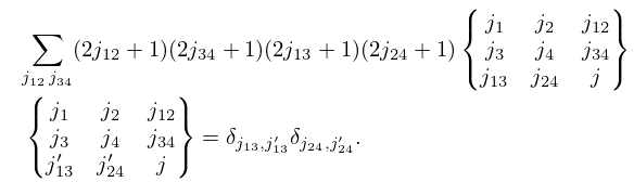
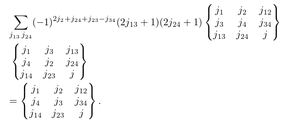
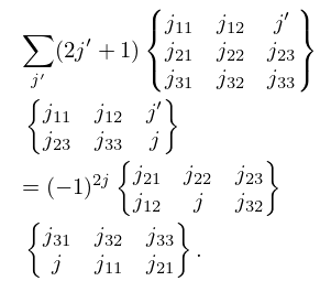
29: 34.7 Basic Properties: $\mathit{9j}$ Symbol

… ►

34.7.1

\begin{Bmatrix}j_{11}&j_{12}&j_{13}\\ j_{21}&j_{22}&j_{13}\\ j_{31}&j_{31}&0\end{Bmatrix}=\frac{(-1)^{j_{12}+j_{21}+j_{13}+j_{31}}}{((2j_{1% 3}+1)(2j_{31}+1))^{\frac{1}{2}}}\begin{Bmatrix}j_{11}&j_{12}&j_{13}\\ j_{22}&j_{21}&j_{31}\end{Bmatrix}.

ⓘ

Symbols:: $\begin{Bmatrix}\NVar{j_{11}}&\NVar{j_{12}}&\NVar{j_{13}}\\ \NVar{j_{21}}&\NVar{j_{22}}&\NVar{j_{23}}\\ \NVar{j_{31}}&\NVar{j_{32}}&\NVar{j_{33}}\end{Bmatrix}$ : $\mathit{9j}$ symbol, $\begin{Bmatrix}\NVar{j_{1}}&\NVar{j_{2}}&\NVar{j_{3}}\\ \NVar{l_{1}}&\NVar{l_{2}}&\NVar{l_{3}}\end{Bmatrix}$ : $\mathit{6j}$ symbol and $j,j_{r}$ : non-negative integers or non-negative integers plus one half.
Permalink:: http://dlmf.nist.gov/34.7.E1
Encodings:: pMML, png, TeX
See also:: Annotations for §34.7(i), §34.7 and Ch.34

… ►

34.7.2

\sum_{j_{12}\,j_{34}}(2j_{12}+1)(2j_{34}+1)(2j_{13}+1)(2j_{24}+1)\begin{% Bmatrix}j_{1}&j_{2}&j_{12}\\ j_{3}&j_{4}&j_{34}\\ j_{13}&j_{24}&j\end{Bmatrix}\begin{Bmatrix}j_{1}&j_{2}&j_{12}\\ j_{3}&j_{4}&j_{34}\\ j^{\prime}_{13}&j^{\prime}_{24}&j\end{Bmatrix}=\delta_{j_{13},j^{\prime}_{13}}% \delta_{j_{24},j^{\prime}_{24}}.

ⓘ

Symbols:: $\delta_{\NVar{j},\NVar{k}}$ : Kronecker delta, $\begin{Bmatrix}\NVar{j_{11}}&\NVar{j_{12}}&\NVar{j_{13}}\\ \NVar{j_{21}}&\NVar{j_{22}}&\NVar{j_{23}}\\ \NVar{j_{31}}&\NVar{j_{32}}&\NVar{j_{33}}\end{Bmatrix}$ : $\mathit{9j}$ symbol and $j,j_{r}$ : non-negative integers or non-negative integers plus one half.
Permalink:: http://dlmf.nist.gov/34.7.E2
Encodings:: pMML, png, TeX
See also:: Annotations for §34.7(iv), §34.7 and Ch.34

… ►

34.7.3

\sum_{j_{13}\,j_{24}}(-1)^{2j_{2}+j_{24}+j_{23}-j_{34}}(2j_{13}+1)(2j_{24}+1)% \begin{Bmatrix}j_{1}&j_{2}&j_{12}\\ j_{3}&j_{4}&j_{34}\\ j_{13}&j_{24}&j\end{Bmatrix}\begin{Bmatrix}j_{1}&j_{3}&j_{13}\\ j_{4}&j_{2}&j_{24}\\ j_{14}&j_{23}&j\end{Bmatrix}=\begin{Bmatrix}j_{1}&j_{2}&j_{12}\\ j_{4}&j_{3}&j_{34}\\ j_{14}&j_{23}&j\end{Bmatrix}.

ⓘ

Symbols:: $\begin{Bmatrix}\NVar{j_{11}}&\NVar{j_{12}}&\NVar{j_{13}}\\ \NVar{j_{21}}&\NVar{j_{22}}&\NVar{j_{23}}\\ \NVar{j_{31}}&\NVar{j_{32}}&\NVar{j_{33}}\end{Bmatrix}$ : $\mathit{9j}$ symbol and $j,j_{r}$ : non-negative integers or non-negative integers plus one half.
Referenced by:: §34.9
Permalink:: http://dlmf.nist.gov/34.7.E3
Encodings:: pMML, png, TeX
See also:: Annotations for §34.7(vi), §34.7 and Ch.34

… ►

34.7.4

\begin{pmatrix}j_{13}&j_{23}&j_{33}\\ m_{13}&m_{23}&m_{33}\end{pmatrix}\begin{Bmatrix}j_{11}&j_{12}&j_{13}\\ j_{21}&j_{22}&j_{23}\\ j_{31}&j_{32}&j_{33}\end{Bmatrix}=\sum_{m_{r1},m_{r2},r=1,2,3}\begin{pmatrix}j% _{11}&j_{12}&j_{13}\\ m_{11}&m_{12}&m_{13}\end{pmatrix}\begin{pmatrix}j_{21}&j_{22}&j_{23}\\ m_{21}&m_{22}&m_{23}\end{pmatrix}\*\begin{pmatrix}j_{31}&j_{32}&j_{33}\\ m_{31}&m_{32}&m_{33}\end{pmatrix}\begin{pmatrix}j_{11}&j_{21}&j_{31}\\ m_{11}&m_{21}&m_{31}\end{pmatrix}\begin{pmatrix}j_{12}&j_{22}&j_{32}\\ m_{12}&m_{22}&m_{32}\end{pmatrix}.

ⓘ

Symbols:: $\begin{Bmatrix}\NVar{j_{11}}&\NVar{j_{12}}&\NVar{j_{13}}\\ \NVar{j_{21}}&\NVar{j_{22}}&\NVar{j_{23}}\\ \NVar{j_{31}}&\NVar{j_{32}}&\NVar{j_{33}}\end{Bmatrix}$ : $\mathit{9j}$ symbol, $\begin{pmatrix}\NVar{j_{1}}&\NVar{j_{2}}&\NVar{j_{3}}\\ \NVar{m_{1}}&\NVar{m_{2}}&\NVar{m_{3}}\end{pmatrix}$ : $\mathit{3j}$ symbol, $j,j_{r}$ : non-negative integers or non-negative integers plus one half. and $r$ : nonnegative integer
Referenced by:: Erratum (V1.0.10) for Equation (34.7.4)
Permalink:: http://dlmf.nist.gov/34.7.E4
Encodings:: pMML, png, TeX
Errata (effective with 1.0.10):: Originally the third $\mathit{3j}$ symbol in the summation was written incorrectly as $\begin{pmatrix}j_{31}&j_{32}&j_{33}\\ m_{13}&m_{23}&m_{33}\end{pmatrix}.$
Reported 2015-01-19 by Yan-Rui Liu
See also:: Annotations for §34.7(vi), §34.7 and Ch.34

►

34.7.5

\sum_{j^{\prime}}(2j^{\prime}+1)\begin{Bmatrix}j_{11}&j_{12}&j^{\prime}\\ j_{21}&j_{22}&j_{23}\\ j_{31}&j_{32}&j_{33}\end{Bmatrix}\begin{Bmatrix}j_{11}&j_{12}&j^{\prime}\\ j_{23}&j_{33}&j\end{Bmatrix}={(-1)^{2j}}\begin{Bmatrix}j_{21}&j_{22}&j_{23}\\ j_{12}&j&j_{32}\end{Bmatrix}\begin{Bmatrix}j_{31}&j_{32}&j_{33}\\ j&j_{11}&j_{21}\end{Bmatrix}.

ⓘ

Symbols:: $\begin{Bmatrix}\NVar{j_{11}}&\NVar{j_{12}}&\NVar{j_{13}}\\ \NVar{j_{21}}&\NVar{j_{22}}&\NVar{j_{23}}\\ \NVar{j_{31}}&\NVar{j_{32}}&\NVar{j_{33}}\end{Bmatrix}$ : $\mathit{9j}$ symbol, $\begin{Bmatrix}\NVar{j_{1}}&\NVar{j_{2}}&\NVar{j_{3}}\\ \NVar{l_{1}}&\NVar{l_{2}}&\NVar{l_{3}}\end{Bmatrix}$ : $\mathit{6j}$ symbol and $j,j_{r}$ : non-negative integers or non-negative integers plus one half.
Permalink:: http://dlmf.nist.gov/34.7.E5
Encodings:: pMML, png, TeX
See also:: Annotations for §34.7(vi), §34.7 and Ch.34

30: 9.18 Tables

… ►

•

Miller (1946) tabulates $\operatorname{Ai}\left(x\right)$ , $\operatorname{Ai}'\left(x\right)$ for $x=-20(.01)2;$ $\operatorname{log}_{10}\operatorname{Ai}\left(x\right)$ , $\operatorname{Ai}'\left(x\right)/\operatorname{Ai}\left(x\right)$ for $x=0(.1)25(1)75$ ; $\operatorname{Bi}\left(x\right)$ , $\operatorname{Bi}'\left(x\right)$ for $x=-10(.1)2.5$ ; $\operatorname{log}_{10}\operatorname{Bi}\left(x\right)$ , $\operatorname{Bi}'\left(x\right)/\operatorname{Bi}\left(x\right)$ for $x=0(.1)10$ ; $M\left(x\right)$ , $N\left(x\right)$ , $\theta\left(x\right)$ , $\phi\left(x\right)$ (respectively $F(x)$ , $G(x)$ , $\chi(x)$ , $\psi(x)$ ) for $x=-80(1)-30(.1)0$ . Precision is generally 8D; slightly less for some of the auxiliary functions. Extracts from these tables are included in Abramowitz and Stegun (1964, Chapter 10), together with some auxiliary functions for large arguments.

… ►

•

National Bureau of Standards (1958) tabulates $A_{0}(x)\equiv\pi\operatorname{Hi}\left(-x\right)$ and $-A_{0}^{\prime}(x)\equiv\pi\operatorname{Hi}'\left(-x\right)$ for $x=0(.01)1(.02)5(.05)11$ and $1/x=0.01(.01)0.1$ ; $\int_{0}^{x}A_{0}(t)\,\mathrm{d}t$ for $x=0.5,1(1)11$ . Precision is 8D.

… ►

•

Gil et al. (2003c) tabulates the only positive zero of $\operatorname{Gi}'\left(z\right)$ , the first 10 negative real zeros of $\operatorname{Gi}\left(z\right)$ and $\operatorname{Gi}'\left(z\right)$ , and the first 10 complex zeros of $\operatorname{Gi}\left(z\right)$ , $\operatorname{Gi}'\left(z\right)$ , $\operatorname{Hi}\left(z\right)$ , and $\operatorname{Hi}'\left(z\right)$ . Precision is 11 or 12S.

…