19 Elliptic Integrals Computation 19.35 Other Applications 19.37 Tables

§19.36 Methods of Computation

Keywords:: symmetric elliptic integrals
Permalink:: http://dlmf.nist.gov/19.36

§19.36(i) Duplication Method
§19.36(ii) Quadratic Transformations
§19.36(iii) Via Theta Functions
§19.36(iv) Other Methods

§19.36(i) Duplication Method

Referenced by:: §19.15, §19.21(ii)
Permalink:: http://dlmf.nist.gov/19.36.i

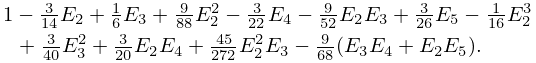
Numerical differences between the variables of a symmetric integral can be reduced in magnitude by successive factors of 4 by repeated applications of the duplication theorem, as shown by (19.26.18). When the differences are moderately small, the iteration is stopped, the elementary symmetric functions of certain differences are calculated, and a polynomial consisting of a fixed number of terms of the sum in (19.19.7) is evaluated. For $\mathop{R_{F}\/}\nolimits$ the polynomial of degree 7, for example, is

19.36.1 $1-\tfrac{1}{10}E_{2}+\tfrac{1}{14}E_{3}+\tfrac{1}{24}E_{2}^{2}-\tfrac{3}{44}E_% {2}E_{3}-\tfrac{5}{208}E_{2}^{3}+\tfrac{3}{104}E_{3}^{2}+\tfrac{1}{16}E_{2}^{2% }E_{3},$

Symbols:: $E_{s}(\mathbf{z})$ : elementary symmetric function
Referenced by:: §19.19, ¶ ‣ §19.36(i), §19.36(i)
Permalink:: http://dlmf.nist.gov/19.36.E1
Encodings:: TeX, pMML, png

where the elementary symmetric functions $E_{s}$ are defined by (19.19.4). If (19.36.1) is used instead of its first five terms, then the factor $(3r)^{{-1/6}}$ in Carlson (1995, (2.2)) is changed to $(3r)^{{-1/8}}$ .

For both $\mathop{R_{D}\/}\nolimits$ and $\mathop{R_{J}\/}\nolimits$ the factor $(r/4)^{{-1/6}}$ in Carlson (1995, (2.18)) is changed to $(r/5)^{{-1/8}}$ when the following polynomial of degree 7 (the same for both) is used instead of its first seven terms:

19.36.2 $1-\tfrac{3}{14}E_{2}+\tfrac{1}{6}E_{3}+\tfrac{9}{88}E_{2}^{2}-\tfrac{3}{22}E_{% 4}-\tfrac{9}{52}E_{2}E_{3}+\tfrac{3}{26}E_{5}-\tfrac{1}{16}E_{2}^{3}+\tfrac{3}% {40}E_{3}^{2}+\tfrac{3}{20}E_{2}E_{4}+\tfrac{45}{272}E_{2}^{2}E_{3}-\tfrac{9}{% 68}(E_{3}E_{4}+E_{2}E_{5}).$

Symbols:: $E_{s}(\mathbf{z})$ : elementary symmetric function
Referenced by:: §19.19
Permalink:: http://dlmf.nist.gov/19.36.E2
Encodings:: TeX, pMML, png

Polynomials of still higher degree can be obtained from (19.19.5) and (19.19.7).

The duplication method starts with computation of $\lambda_{0}=\sqrt{x}\sqrt{y}+\sqrt{y}\sqrt{z}+\sqrt{z}\sqrt{x}$ . The reductions in §19.29(i) represent as squares, for example $x=U_{{12}}^{2}$ in (19.29.4). Because $U_{{12}}$ may be real and negative, or even complex, care is needed to ensure $\sqrt{x}=U_{{12}}$ , and similarly for and . This precaution is needed only for $\lambda_{0}$ . Alternatively, the first duplication is done analytically as in Carlson and FitzSimons (2000), where further information can be found.

¶ Example

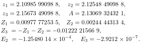
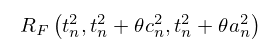
Keywords:: Legendre’s elliptic integrals

Three applications of (19.26.18) yield

19.36.3 $\mathop{R_{F}\/}\nolimits\!\left(1,2,4\right)=\mathop{R_{F}\/}\nolimits\!\left% (z_{1},z_{2},z_{3}\right),$

Symbols:: $\mathop{R_{F}\/}\nolimits\!\left(x,y,z\right)$ : symmetric elliptic integral of first kind
Permalink:: http://dlmf.nist.gov/19.36.E3
Encodings:: TeX, pMML, png

where, in the notation of (19.19.7) with $a=-\frac{1}{2}$ and ,

19.36.4 $\begin{aligned}\displaystyle z_{1}&\displaystyle=2.10985\;99098\;8,\\ \displaystyle z_{3}&\displaystyle=2.15673\;49098\;8,\\ \displaystyle Z_{1}&\displaystyle=0.00977\;77253\;5,\end{aligned}\quad\begin{% aligned}\displaystyle z_{2}&\displaystyle=2.12548\;49098\;8,\\ \displaystyle A&\displaystyle=2.13069\;32432\;1,\\ \displaystyle Z_{2}&\displaystyle=0.00244\;44313\;4,\end{aligned}\\ {Z_{3}=-Z_{1}-Z_{2}=-0.01222\;21566\;9,}\\ {E_{2}=\Sci{-1.25480\;14}{-4},\quad E_{3}=\Sci{-2.9212}{-7}.}$

Symbols:: $E_{s}(\mathbf{z})$ : elementary symmetric function, $Z_{j}$ : components and
Permalink:: http://dlmf.nist.gov/19.36.E4
Encodings:: TeX, pMML, png

The first five terms of (19.36.1) suffice for

19.36.5 $\mathop{R_{F}\/}\nolimits\!\left(1,2,4\right)=0.68508\;58166\dots.$

Symbols:: $\mathop{R_{F}\/}\nolimits\!\left(x,y,z\right)$ : symmetric elliptic integral of first kind
Referenced by:: ¶ ‣ §19.36(ii)
Permalink:: http://dlmf.nist.gov/19.36.E5
Encodings:: TeX, pMML, png

All cases of $\mathop{R_{F}\/}\nolimits$ , $\mathop{R_{C}\/}\nolimits$ , $\mathop{R_{J}\/}\nolimits$ , and $\mathop{R_{D}\/}\nolimits$ are computed by essentially the same procedure (after transforming Cauchy principal values by means of (19.20.14) and (19.2.20)). Complex values of the variables are allowed, with some restrictions in the case of $\mathop{R_{J}\/}\nolimits$ that are sufficient but not always necessary. The computation is slowest for complete cases. For details see Carlson (1995, 2002) and Carlson and FitzSimons (2000). In the Appendix of the last reference it is shown how to compute $\mathop{R_{J}\/}\nolimits$ without computing $\mathop{R_{C}\/}\nolimits$ more than once. Because of cancellations in (19.26.21) it is advisable to compute $\mathop{R_{G}\/}\nolimits$ from $\mathop{R_{F}\/}\nolimits$ and $\mathop{R_{D}\/}\nolimits$ by (19.21.10) or else to use §19.36(ii).

Legendre’s integrals can be computed from symmetric integrals by using the relations in §19.25(i). Note the remark following (19.25.11). If (19.25.9) is used when $0\leq k^{2}\leq 1$ , cancellations may lead to loss of significant figures when $k^{2}$ is close to 1 and $\phi>\pi/4$ , as shown by Reinsch and Raab (2000). The cancellations can be eliminated, however, by using (19.25.10).

Accurate values of $\mathop{F\/}\nolimits\!\left(\phi,k\right)-\mathop{E\/}\nolimits\!\left(\phi,k\right)$ for $k^{2}$ near 0 can be obtained from $\mathop{R_{D}\/}\nolimits$ by (19.2.6) and (19.25.13).

§19.36(ii) Quadratic Transformations

Notes:: See Carlson (1965, (3.1), (3.2), Sections 5, 6). To obtain (19.36.6) and (19.36.8) from (19.22.18), let $(x^{2},y^{2},z^{2})=(t_{n}^{2},t_{n}^{2}+\theta c_{n}^{2},t_{n}^{2}+\theta a_{% n}^{2})$ and $(a^{2},z_{{-}}^{2},z_{{+}}^{2})=(t_{{n+1}}^{2},t_{{n+1}}^{2}+\theta c_{{n+1}}^% {2},t_{{n+1}}^{2}+\theta a_{{n+1}}^{2})$ . Then use the expression for $z_{{\pm}}^{2}-a^{2}$ from (19.22.17) and the definition of from (19.22.16).
Referenced by:: ¶ ‣ §19.36(i)
Permalink:: http://dlmf.nist.gov/19.36.ii

Complete cases of Legendre’s integrals and symmetric integrals can be computed with quadratic convergence by the AGM method (including Bartky transformations), using the equations in §19.8(i) and §19.22(ii), respectively.

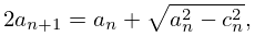
The incomplete integrals $\mathop{R_{F}\/}\nolimits\!\left(x,y,z\right)$ and $\mathop{R_{G}\/}\nolimits\!\left(x,y,z\right)$ can be computed by successive transformations in which two of the three variables converge quadratically to a common value and the integrals reduce to $\mathop{R_{C}\/}\nolimits$ , accompanied by two quadratically convergent series in the case of $\mathop{R_{G}\/}\nolimits$ ; compare Carlson (1965, §§5,6). (In Legendre’s notation the modulus approaches 0 or 1.) Let

19.36.6

$2a_{{n+1}}=a_{n}+\sqrt{a_{n}^{2}-c_{n}^{2}},$

$2c_{{n+1}}=a_{n}-\sqrt{a_{n}^{2}-c_{n}^{2}}=c_{n}^{2}/(2a_{{n+1}}),$

$2t_{{n+1}}=t_{n}+\sqrt{t_{n}^{2}+\theta c_{n}^{2}},$

Symbols:: : nonnegative integer
Referenced by:: ¶ ‣ §19.36(ii), §19.36(ii)
Permalink:: http://dlmf.nist.gov/19.36.E6
Encodings:: TeX, TeX, TeX, pMML, pMML, pMML, png, png, png

where $n=0,1,2,\dots$ , and

19.36.7

$0<c_{0}<a_{0},$

$t_{0}\geq 0,$

$t_{0}^{2}+\theta a_{0}^{2}\geq 0,$

$\theta=\pm 1.$

Permalink:: http://dlmf.nist.gov/19.36.E7
Encodings:: TeX, TeX, TeX, TeX, pMML, pMML, pMML, pMML, png, png, png, png

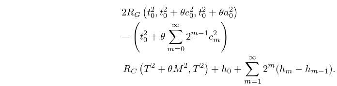
Then (19.22.18) implies that

19.36.8 $\mathop{R_{F}\/}\nolimits\!\left(t_{n}^{2},t_{n}^{2}+\theta c_{n}^{2},t_{n}^{2% }+\theta a_{n}^{2}\right)$

Symbols:: $\mathop{R_{F}\/}\nolimits\!\left(x,y,z\right)$ : symmetric elliptic integral of first kind and : nonnegative integer
Referenced by:: §19.36(ii)
Permalink:: http://dlmf.nist.gov/19.36.E8
Encodings:: TeX, pMML, png

is independent of . As $n\to\infty$ , $c_{n}$ , $a_{n}$ , and $t_{n}$ converge quadratically to limits 0, , and , respectively; hence

19.36.9 $\mathop{R_{F}\/}\nolimits\!\left(t_{0}^{2},t_{0}^{2}+\theta c_{0}^{2},t_{0}^{2% }+\theta a_{0}^{2}\right)=\mathop{R_{F}\/}\nolimits\!\left(T^{2},T^{2},T^{2}+% \theta M^{2}\right)=\mathop{R_{C}\/}\nolimits\!\left(T^{2}+\theta M^{2},T^{2}% \right).$

Symbols:: $\mathop{R_{C}\/}\nolimits\!\left(x,y\right)$ : Carlson’s combination of inverse circular and inverse hyperbolic functions, $\mathop{R_{F}\/}\nolimits\!\left(x,y,z\right)$ : symmetric elliptic integral of first kind, : limit and : limit
Referenced by:: §19.15
Permalink:: http://dlmf.nist.gov/19.36.E9
Encodings:: TeX, pMML, png

If $t_{0}=a_{0}$ and $\theta=-1$ , so that $t_{n}=a_{n}$ , then this procedure reduces to the AGM method for the complete integral.

The step from to is an ascending Landen transformation if $\theta=1$ (leading ultimately to a hyperbolic case of $\mathop{R_{C}\/}\nolimits$ ) or a descending Gauss transformation if $\theta=-1$ (leading to a circular case of $\mathop{R_{C}\/}\nolimits$ ). If , , and are permuted so that $0\leq x<y<z$ , then the computation of $\mathop{R_{F}\/}\nolimits\!\left(x,y,z\right)$ is fastest if we make $c_{0}^{2}\leq a_{0}^{2}/2$ by choosing $\theta=1$ when or $\theta=-1$ when $y\geq(x+z)/2$ .

¶ Example

Keywords:: Bulirsch’s elliptic integrals

We compute $\mathop{R_{F}\/}\nolimits\!\left(1,2,4\right)$ by setting $\theta=1$ , $t_{0}=c_{0}=1$ , and $a_{0}=\sqrt{3}$ . Then

19.36.10

$c_{3}^{2}=\Sci{6.65}{-12},$

$a_{3}^{2}=2.46209\;30206\;0=M^{2},$

$t_{3}^{2}=1.46971\;53173\;1=T^{2}.$

Symbols:: : limit and : limit
Permalink:: http://dlmf.nist.gov/19.36.E10
Encodings:: TeX, TeX, TeX, pMML, pMML, pMML, png, png, png

Hence

19.36.11 $\mathop{R_{F}\/}\nolimits\!\left(1,2,4\right)=\mathop{R_{C}\/}\nolimits\!\left% (T^{2}+M^{2},T^{2}\right)=0.68508\;58166,$

Symbols:: $\mathop{R_{C}\/}\nolimits\!\left(x,y\right)$ : Carlson’s combination of inverse circular and inverse hyperbolic functions, $\mathop{R_{F}\/}\nolimits\!\left(x,y,z\right)$ : symmetric elliptic integral of first kind, : limit and : limit
Permalink:: http://dlmf.nist.gov/19.36.E11
Encodings:: TeX, pMML, png

in agreement with (19.36.5). Here $\mathop{R_{C}\/}\nolimits$ is computed either by the duplication algorithm in Carlson (1995) or via (19.2.19).

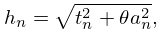
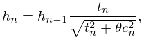
To (19.36.6) add

19.36.12

$h_{n}=\sqrt{t_{n}^{2}+\theta a_{n}^{2}},$ $n=0,1,2,\dots$ ,

$h_{n}=h_{{n-1}}\frac{t_{n}}{\sqrt{t_{n}^{2}+\theta c_{n}^{2}}},$ $n=1,2,\dots$ .

Symbols:: : nonnegative integer and $h_{n}$
Referenced by:: ¶ ‣ §19.36(ii)
Permalink:: http://dlmf.nist.gov/19.36.E12
Encodings:: TeX, TeX, pMML, pMML, png, png

Then

19.36.13 $2\!\mathop{R_{G}\/}\nolimits\!\left(t_{0}^{2},t_{0}^{2}+\theta c_{0}^{2},t_{0}% ^{2}+\theta a_{0}^{2}\right)=\left(t_{0}^{2}+\theta\sum_{{m=0}}^{{\infty}}2^{{% m-1}}c_{m}^{2}\right)\mathop{R_{C}\/}\nolimits\!\left(T^{2}+\theta M^{2},T^{2}% \right)+h_{0}+\sum_{{m=1}}^{{\infty}}2^{m}(h_{m}-h_{{m-1}}).$

Symbols:: $\mathop{R_{C}\/}\nolimits\!\left(x,y\right)$ : Carlson’s combination of inverse circular and inverse hyperbolic functions, $\mathop{R_{G}\/}\nolimits\!\left(x,y,z\right)$ : symmetric elliptic integral of second kind, : nonnegative integer, : limit, : limit and $h_{n}$
Permalink:: http://dlmf.nist.gov/19.36.E13
Encodings:: TeX, pMML, png

If the iteration of (19.36.6) and (19.36.12) is stopped when $c_{s}<\sqrt{r}t_{s}$ ( and being approximated by $a_{s}$ and $t_{s}$ , and the infinite series being truncated), then the relative error in $\mathop{R_{F}\/}\nolimits$ and $\mathop{R_{G}\/}\nolimits$ is less than if we neglect terms of order $r^{2}$ .

$\mathop{F\/}\nolimits\!\left(\phi,k\right)$ can be evaluated by using (19.25.5). $\mathop{E\/}\nolimits\!\left(\phi,k\right)$ can be evaluated by using (19.25.7), and $\mathop{R_{D}\/}\nolimits$ by using (19.21.10), but cancellations may become significant. Thompson (1997, pp. 499, 504) uses descending Landen transformations for both $\mathop{F\/}\nolimits\!\left(\phi,k\right)$ and $\mathop{E\/}\nolimits\!\left(\phi,k\right)$ . A summary for $\mathop{F\/}\nolimits\!\left(\phi,k\right)$ is given in Gautschi (1975, §3). For computation of $\mathop{K\/}\nolimits\!\left(k\right)$ and $\mathop{E\/}\nolimits\!\left(k\right)$ with complex see Fettis and Caslin (1969) and Morita (1978).

(19.22.20) reduces to if or , and (19.22.19) reduces to if or . Near these points there will be loss of significant figures in the computation of $\mathop{R_{J}\/}\nolimits$ or $\mathop{R_{D}\/}\nolimits$ .

Descending Gauss transformations of $\mathop{\Pi\/}\nolimits\!\left(\phi,\alpha^{2},k\right)$ (see (19.8.20)) are used in Fettis (1965) to compute a large table (see §19.37(iii)). This method loses significant figures in $\rho$ if $\alpha^{2}$ and $k^{2}$ are nearly equal unless they are given exact values—as they can be for tables. If $\alpha^{2}=k^{2}$ , then the method fails, but the function can be expressed by (19.6.13) in terms of $\mathop{E\/}\nolimits\!\left(\phi,k\right)$ , for which Neuman (1969b) uses ascending Landen transformations.

Computation of Legendre’s integrals of all three kinds by quadratic transformation is described by Cazenave (1969, pp. 128–159, 208–230).

Quadratic transformations can be applied to compute Bulirsch’s integrals (§19.2(iii)). The function $\mathop{\mathrm{cel}\/}\nolimits\!\left(k_{c},p,a,b\right)$ is computed by successive Bartky transformations (Bulirsch and Stoer (1968), Bulirsch (1969b)). The function $\mathop{\mathrm{el2}\/}\nolimits\!\left(x,k_{c},a,b\right)$ is computed by descending Landen transformations if is real, or by descending Gauss transformations if is complex (Bulirsch (1965b)). Remedies for cancellation when is real and near 0 are supplied in Midy (1975). See also Bulirsch (1969a) and Reinsch and Raab (2000).

Bulirsch (1969a, b) extend Bartky’s transformation to $\mathop{\mathrm{el3}\/}\nolimits\!\left(x,k_{c},p\right)$ by expressing it in terms of the first incomplete integral, a complete integral of the third kind, and a more complicated integral to which Bartky’s method can be applied. The cases $k_{c}^{2}/2\leq p<\infty$ and $-\infty<p<k_{c}^{2}/2$ require different treatment for numerical purposes, and again precautions are needed to avoid cancellations.

§19.36(iii) Via Theta Functions

Permalink:: http://dlmf.nist.gov/19.36.iii

Lee (1990) compares the use of theta functions for computation of $\mathop{K\/}\nolimits\!\left(k\right)$ , $\mathop{E\/}\nolimits\!\left(k\right)$ , and $\mathop{K\/}\nolimits\!\left(k\right)-\mathop{E\/}\nolimits\!\left(k\right)$ , $0\leq k^{2}\leq 1$ , with four other methods. Also, see Todd (1975) for a special case of $\mathop{K\/}\nolimits\!\left(k\right)$ . For computation of Legendre’s integral of the third kind, see Abramowitz and Stegun (1964, §§17.7 and 17.8, Examples 15, 17, 19, and 20). For integrals of the second and third kinds see Lawden (1989, §§3.4–3.7).

§19.36(iv) Other Methods

Keywords:: Legendre’s elliptic integrals
Referenced by:: Other Changes
Permalink:: http://dlmf.nist.gov/19.36.iv
Addition (effective with 1.0.5):: The references to Karp and Sitnik (2007) and Fukushima (2010) have been added at the end of this subsection.
Reported 2012-07-30

Numerical quadrature is slower than most methods for the standard integrals but can be useful for elliptic integrals that have complicated representations in terms of standard integrals. See §3.5.

For series expansions of Legendre’s integrals see §19.5. Faster convergence of power series for $\mathop{K\/}\nolimits\!\left(k\right)$ and $\mathop{E\/}\nolimits\!\left(k\right)$ can be achieved by using (19.5.1) and (19.5.2) in the right-hand sides of (19.8.12). A three-part computational procedure for $\mathop{\Pi\/}\nolimits\!\left(\phi,\alpha^{2},k\right)$ is described by Franke (1965) for $\alpha^{2}<1$ .

When the values of complete integrals are known, addition theorems with $\psi=\pi/2$ (§19.11(ii)) ease the computation of functions such as $\mathop{F\/}\nolimits\!\left(\phi,k\right)$ when $\frac{1}{2}\pi-\phi$ is small and positive. Similarly, §19.26(ii) eases the computation of functions such as $\mathop{R_{F}\/}\nolimits\!\left(x,y,z\right)$ when () is small compared with $\min(y,z)$ . These special theorems are also useful for checking computer codes.

For fast methods for computing the incomplete elliptic integral of the first kind see Karp and Sitnik (2007) and Fukushima (2010).

© 2010–2013 NIST / Privacy Policy / Disclaimer / Feedback; Version 1.0.6; Release date 2013-05-06 Math-Image version (See MathML) . A Printed Companionis available. 19.35 Other Applications 19.37 Tables

§19.36 Methods of Computation

Contents

§19.36(i) Duplication Method

¶ Example

§19.36(ii) Quadratic Transformations

¶ Example

§19.36(iii) Via Theta Functions

§19.36(iv) Other Methods