§18.40 Methods of Computation
Contents
§18.40(i) Computation of Polynomials
Orthogonal polynomials can be computed from their explicit polynomial form by Horner’s scheme (§1.11(i)). Usually, however, other methods are more efficient, especially the numerical solution of difference equations (§3.6) and the application of uniform asymptotic expansions (when available) for OP’s of large degree. For applications in which the OP’s appear only as terms in series expansions (compare §18.18(i)) the need to compute them can be avoided altogether by use instead of Clenshaw’s algorithm (§3.11(ii)) and its straightforward generalization to OP’s other than Chebyshev. For further information see Clenshaw (1955), Gautschi (2004, §§2.1, 8.1), and Mason and Handscomb (2003, §2.4).
§18.40(ii) The Classical Moment Problem
The problem of moments is simply stated and the early work of Stieltjes, Markov, and Chebyshev on this problem was the origin of the understanding of the importance of both continued fractions and OP’s in many areas of analysis. Given the power moments, , , can these be used to find a unique , a non-decreasing, real, function of , in the case that the moment problem is determined? Should a unique solution not exist the moment problem is then indeterminant. The theory behind these remarks is in Shohat and Tamarkin (1970), Akhiezer (2021), Chihara (1978).
A numerical approach to the recursion coefficients and quadrature abscissas and weights
In what follows we consider only the simple, illustrative, case that is continuously differentiable so that , with real, positive, and continuous on a real interval The strategy will be to: 1) use the moments to determine the recursion coefficients of equations (18.2.11_5) and (18.2.11_8); then, 2) to construct the quadrature abscissas and weights (or Christoffel numbers) from the J-matrix of §3.5(vi), equations (3.5.31) and(3.5.32). These quadrature weights and abscissas will then allow construction of a convergent sequence of approximations to , as will be considered in the following paragraphs.
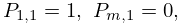
There are many ways to implement these first two steps, noting that the expressions for and of equation (18.2.30) are of little practical numerical value, see Gautschi (2004) and Golub and Meurant (2010). A simple set of choices is spelled out in Gordon (1968) which gives a numerically stable algorithm for direct computation of the recursion coefficients in terms of the moments, followed by construction of the J-matrix and quadrature weights and abscissas, and we will follow this approach: Let be a positive integer and define
| 18.40.1 | ||||
| , | ||||
| , | ||||
| , , , | ||||
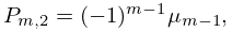
use the first row of this -matrix for
| 18.40.2 | |||
| , | |||
and these can be used for the recursion coefficients
| 18.40.3 | |||
| . | |||
The quadrature abscissas and weights then follow from the discussion of §3.5(vi). See Gautschi (1983) for examples of numerically stable and unstable use of the above recursion relations, and how one can then usefully differentiate between numerical results of low and high precision, as produced thereby.
Having now directly connected computation of the quadrature abscissas and weights to the moments, what follows uses these for a Stieltjes–Perron inversion to regain .
Stieltjes Inversion via (approximate) Analytic Continuation
We have from (18.2.38) that
| 18.40.4 | |||
| , | |||
in which
| 18.40.5 | |||
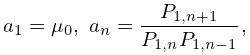
Let . It is now necessary to take the limit of , and the imaginary part is the required Stieltjes–Perron inversion:
| 18.40.6 | |||
The question is then: how is this possible given only , rather than itself? often converges to smooth results for off the real axis for at a distance greater than the pole spacing of the , this may then be followed by approximate numerical analytic continuation via fitting to lower order continued fractions (either Padé, see §3.11(iv), or pointwise continued fraction approximants, see Schlessinger (1968, Appendix)), to and evaluating these on the real axis in regions of higher pole density that those of the approximating function. Results of low ( to decimal digits) precision for are easily obtained for to . Gautschi (2004, p. 119–120) has explored the limit via the Wynn -algorithm, (3.9.11) to accelerate convergence, finding four to eight digits of precision in , depending smoothly on , for , for an example involving first numerator Legendre OP’s.
Histogram Approach
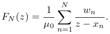
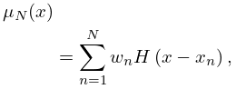
The quadrature points and weights can be put to a more direct and efficient use. Define
| 18.40.7 | |||
| , | |||
being the Heaviside step-function, see (1.16.13).
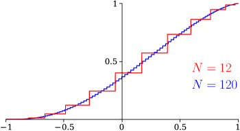
Equation (18.40.7) provides step-histogram approximations to , as shown in Figure 18.40.1 for and , shown here for the repulsive Coulomb–Pollaczek OP’s of Figure 18.39.2, with the parameters as listed therein.

The bottom and top of the steps at the are lower and upper bounds to as made explicit via the Chebyshev inequalities discussed by Shohat and Tamarkin (1970, pp. 42–43). Interpolation of the midpoints of the jumps followed by differentiation with respect to yields a Stieltjes–Perron inversion to obtain to a precision of decimal digits for . Convergence is . Results similar to these appear in Langhoff et al. (1976) in methods developed for physics applications, and which includes treatments of systems with discontinuities in , using what is referred to as the Stieltjes derivative which may be traced back to Stieltjes, as discussed by Deltour (1968, Eq. 12).
Derivative Rule Approach
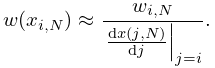
An alternate, and highly efficient, approach follows from the derivative rule conjecture, see Yamani and Reinhardt (1975), and references therein, namely that
| 18.40.8 | |||
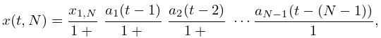
This allows Stieltjes–Perron inversion for the , given the quadrature weights and points. Here is an interpolation of the abscissas , that is, , allowing differentiation by . In what follows this is accomplished in two ways: i) via the Lagrange interpolation of §3.3(i) ; and ii) by constructing a pointwise continued fraction, or PWCF, as follows:
| 18.40.9 | |||
| , | |||
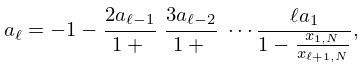
where the coefficients are defined recursively via , and
| 18.40.10 | |||
| . | |||
The PWCF is a minimally oscillatory algebraic interpolation of the abscissas .
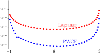
Comparisons of the precisions of Lagrange and PWCF interpolations to obtain the derivatives, are shown in Figure 18.40.2. The example chosen is inversion from the for the weight function for the repulsive Coulomb–Pollaczek, RCP, polynomials of (18.39.50). This is a challenging case as the desired on has an essential singularity at .

Further, exponential convergence in , via the Derivative Rule, rather than the power-law convergence of the histogram methods, is found for the inversion of Gegenbauer, Attractive, as well as Repulsive, Coulomb–Pollaczek, and Hermite weights and zeros to approximate for these OP systems on and respectively, Reinhardt (2018), and Reinhardt (2021b), Reinhardt (2021a). Achieving precisions at this level shown above requires higher than normal computational precision, see Gautschi (2009). In Figure 18.40.2 the approximations were carried out with a precision of 50 decimal digits.
