§13.29 Methods of Computation

Referenced by:: §12.18, §16.25, §33.23(i)
Permalink:: http://dlmf.nist.gov/13.29

§13.29(i) Series Expansions
§13.29(ii) Differential Equations
§13.29(iii) Integral Representations
§13.29(iv) Recurrence Relations

§13.29(i) Series Expansions

Permalink:: http://dlmf.nist.gov/13.29.i

Although the Maclaurin series expansion (13.2.2) converges for all finite values of $z$ , it is cumbersome to use when $|z|$ is large owing to slowness of convergence and cancellation. For large $|z|$ the asymptotic expansions of §13.7 should be used instead. Accuracy is limited by the magnitude of $|z|$ . However, this accuracy can be increased considerably by use of the exponentially-improved forms of expansion supplied by the combination of (13.7.10) and (13.7.11), or by use of the hyperasymptotic expansions given in Olde Daalhuis and Olver (1995a). For large values of the parameters $a$ and $b$ the approximations in §13.8 are available.

Similarly for the Whittaker functions.

§13.29(ii) Differential Equations

Permalink:: http://dlmf.nist.gov/13.29.ii

A comprehensive and powerful approach is to integrate the differential equations (13.2.1) and (13.14.1) by direct numerical methods. As described in §3.7(ii), to insure stability the integration path must be chosen in such a way that as we proceed along it the wanted solution grows in magnitude at least as fast as all other solutions of the differential equation.

For $\mathop{M\/}\nolimits\!\left(a,b,z\right)$ and $\mathop{M_{{\kappa,\mu}}\/}\nolimits\!\left(z\right)$ this means that in the sector $|\mathop{\mathrm{ph}\/}\nolimits z|\leq\pi$ we may integrate along outward rays from the origin with initial values obtained from (13.2.2) and (13.14.2).

For $\mathop{U\/}\nolimits\!\left(a,b,z\right)$ and $\mathop{W_{{\kappa,\mu}}\/}\nolimits\!\left(z\right)$ we may integrate along outward rays from the origin in the sectors $\tfrac{1}{2}\pi<|\mathop{\mathrm{ph}\/}\nolimits z|<\tfrac{3}{2}\pi$ , with initial values obtained from connection formulas in §13.2(vii), §13.14(vii). In the sector $|\mathop{\mathrm{ph}\/}\nolimits z|<\tfrac{1}{2}\pi$ the integration has to be towards the origin, with starting values computed from asymptotic expansions (§§13.7 and 13.19). On the rays $\mathop{\mathrm{ph}\/}\nolimits z=\pm\tfrac{1}{2}\pi$ , integration can proceed in either direction.

§13.29(iii) Integral Representations

Permalink:: http://dlmf.nist.gov/13.29.iii

The integral representations (13.4.1) and (13.4.4) can be used to compute the Kummer functions, and (13.16.1) and (13.16.5) for the Whittaker functions. In Allasia and Besenghi (1991) and Allasia and Besenghi (1987a) the high accuracy of the trapezoidal rule for the computation of Kummer functions is described. Gauss quadrature methods are discussed in Gautschi (2002b).

§13.29(iv) Recurrence Relations

Permalink:: http://dlmf.nist.gov/13.29.iv

The recurrence relations in §§13.3(i) and 13.15(i) can be used to compute the confluent hypergeometric functions in an efficient way. In the following two examples Olver’s algorithm (§3.6(v)) can be used.

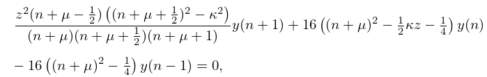
¶ Example 1

We assume $2\mu\neq-1,-2,-3,\dots$ . Then we have

13.29.1 $\frac{z^{2}(n+\mu-\tfrac{1}{2})\left((n+\mu+\tfrac{1}{2})^{2}-\kappa^{2}\right)}{(n+\mu)(n+\mu+\tfrac{1}{2})(n+\mu+1)}{y(n+1)}+16\left((n+\mu)^{2}-\tfrac{1}{2}\kappa z-\tfrac{1}{4}\right)y(n)\\ -16\left((n+\mu)^{2}-\tfrac{1}{4}\right)y(n-1)=0,$

Symbols:: $n$ : nonnegative integer, $z$ : complex variable and $y(n)$ : solution
Permalink:: http://dlmf.nist.gov/13.29.E1
Encodings:: TeX, pMML, png

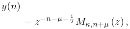
with recessive solution

13.29.2 $y(n)=z^{{-n-\mu-\frac{1}{2}}}\mathop{M_{{\kappa,n+\mu}}\/}\nolimits\!\left(z\right),$

Symbols:: $\mathop{M_{{\kappa,\mu}}\/}\nolimits\!\left(z\right)$ : Whittaker confluent hypergeometric function, $n$ : nonnegative integer, $z$ : complex variable and $y(n)$ : solution
Permalink:: http://dlmf.nist.gov/13.29.E2
Encodings:: TeX, pMML, png

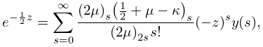
normalizing relation

13.29.3 $e^{{-\frac{1}{2}z}}=\sum _{{s=0}}^{{\infty}}\frac{\left(2\mu\right)_{{s}}\left(\frac{1}{2}+\mu-\kappa\right)_{{s}}}{\left(2\mu\right)_{{2s}}s!}(-z)^{s}y(s),$

Symbols:: $\left(a\right)_{{n}}$ : Pochhammer’s symbol, $e$ : base of exponential function, $!$ : $n!$ : factorial, $s$ : nonnegative integer, $z$ : complex variable and $y(n)$ : solution
Permalink:: http://dlmf.nist.gov/13.29.E3
Encodings:: TeX, pMML, png

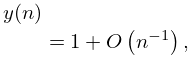
and estimate

13.29.4 $y(n)=1+\mathop{O\/}\nolimits\!\left(n^{{-1}}\right),$ $n\to\infty$ .

Symbols:: $\mathop{O\/}\nolimits\!\left(x\right)$ : order not exceeding, $n$ : nonnegative integer and $y(n)$ : solution
Permalink:: http://dlmf.nist.gov/13.29.E4
Encodings:: TeX, pMML, png

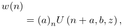
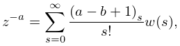
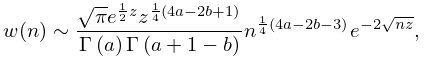
¶ Example 2

We assume $a,a+1-b\neq 0,-1,-2,\dots$ . Then we have

13.29.5 $(n+a)w(n)-\left(2(n+a+1)+z-b\right)w(n+1)+(n+a-b+2)w(n+2)=0,$

Symbols:: $n$ : nonnegative integer and $z$ : complex variable
Permalink:: http://dlmf.nist.gov/13.29.E5
Encodings:: TeX, pMML, png

with recessive solution

13.29.6 $w(n)=\left(a\right)_{{n}}\mathop{U\/}\nolimits\!\left(n+a,b,z\right),$

Symbols:: $\mathop{U\/}\nolimits\!\left(a,b,z\right)$ : Kummer confluent hypergeometric function, $\left(a\right)_{{n}}$ : Pochhammer’s symbol, $n$ : nonnegative integer and $z$ : complex variable
Permalink:: http://dlmf.nist.gov/13.29.E6
Encodings:: TeX, pMML, png

normalizing relation

13.29.7 $z^{{-a}}=\sum _{{s=0}}^{{\infty}}\frac{\left(a-b+1\right)_{{s}}}{s!}w(s),$

Symbols:: $\left(a\right)_{{n}}$ : Pochhammer’s symbol, $!$ : $n!$ : factorial, $s$ : nonnegative integer and $z$ : complex variable
Permalink:: http://dlmf.nist.gov/13.29.E7
Encodings:: TeX, pMML, png