§3.5 Quadrature
Contents
- §3.5(i) Trapezoidal Rules
- §3.5(ii) Simpson’s Rule
- §3.5(iii) Romberg Integration
- §3.5(iv) Interpolatory Quadrature Rules
- §3.5(v) Gauss Quadrature
- §3.5(vi) Eigenvalue/Eigenvector Characterization of Gauss Quadrature Formulas
- §3.5(vii) Oscillatory Integrals
- §3.5(viii) Complex Gauss Quadrature
- §3.5(ix) Other Contour Integrals
- §3.5(x) Cubature Formulas
§3.5(i) Trapezoidal Rules
The elementary trapezoidal rule is given by
| 3.5.1 | |||
where , , and .
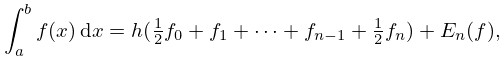
The composite trapezoidal rule is
| 3.5.2 | |||
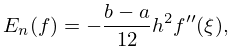
where , , , , and
| 3.5.3 | |||
| . | |||
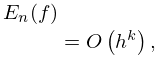
If in addition is periodic, , and the integral is taken over a period, then
| 3.5.4 | |||
| . | |||
In particular, when the error term is an exponentially-small function of , and in these circumstances the composite trapezoidal rule is exceptionally efficient. For an example see §3.5(ix).
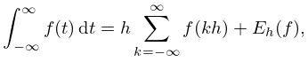
Similar results hold for the trapezoidal rule in the form
| 3.5.5 | |||
with a function that is analytic in a strip containing . For further information and examples, see Goodwin (1949b). In Stenger (1993, Chapter 3) the rule (3.5.5) is considered in the framework of Sinc approximations (§3.3(vi)). See also Poisson’s summation formula (§1.8(iv)).
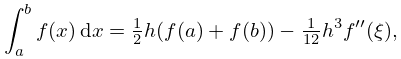
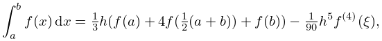
§3.5(ii) Simpson’s Rule
Let and . Then the elementary Simpson’s rule is
| 3.5.6 | |||
where .
Now let , , and , . Then the composite Simpson’s rule is
| 3.5.7 | |||
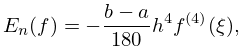
where is even and
| 3.5.8 | |||
| . | |||
Simpson’s rule can be regarded as a combination of two trapezoidal rules, one with step size and one with step size to refine the error term.
§3.5(iii) Romberg Integration
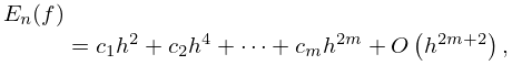
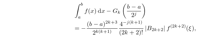
Further refinements are achieved by Romberg integration. If , then the remainder in (3.5.2) can be expanded in the form
| 3.5.9 | |||
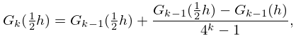
where . As in Simpson’s rule, by combining the rule for with that for , the first error term in (3.5.9) can be eliminated. With the Romberg scheme successive terms , in (3.5.9) are eliminated, according to the formula
| 3.5.10 | |||
| , | |||
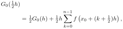
beginning with
| 3.5.11 | |||
although we may also start with the elementary rule with and . To generate the quantities are needed. These can be found by means of the recursion
| 3.5.12 | |||
which depends on function values computed previously.
When , the Romberg method affords a means of obtaining high accuracy in many cases with a relatively simple adaptive algorithm. However, as illustrated by the next example, other methods may be more efficient.
Example
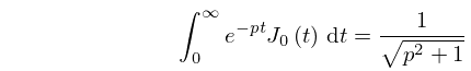
With denoting the Bessel function (§10.2(ii)) the integral
| 3.5.14 | |||
is computed with on the interval . Using (3.5.10) with we obtain with 14 correct digits. About function evaluations are needed. (With the 20-point Gauss–Laguerre formula (§3.5(v)) the same precision can be achieved with 15 function evaluations.) With and , the coefficient of the derivative in (3.5.13) is found to be .
See Davis and Rabinowitz (1984, pp. 440–441) for modifications of the Romberg method when the function is singular.
§3.5(iv) Interpolatory Quadrature Rules
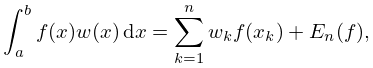
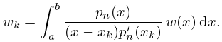
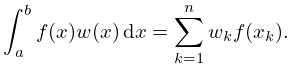
An interpolatory quadrature rule
| 3.5.15 | |||
with weight function , is one for which whenever is a polynomial of degree . The nodes are prescribed, and the weights and error term are found by integrating the product of the Lagrange interpolation polynomial of degree and .
If the extreme members of the set of nodes are the endpoints and , then the quadrature rule is said to be closed. Or if the set lies in the open interval , then the quadrature rule is said to be open.
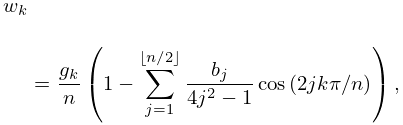
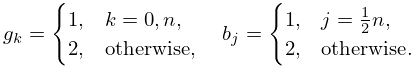
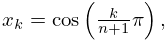
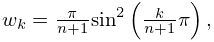
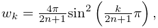
Rules of closed type include the Newton–Cotes formulas such as the trapezoidal rules and Simpson’s rule. Examples of open rules are the Gauss formulas (§3.5(v)), the midpoint rule, and Fejér’s quadrature rule. For the latter , , and the nodes are the extrema of the Chebyshev polynomial (§3.11(ii) and §18.3). If we add and to this set of , then the resulting closed formula is the frequently-used Clenshaw–Curtis formula, whose weights are positive and given by
| 3.5.16 | |||
where , and
| 3.5.17 | |||
§3.5(v) Gauss Quadrature
Let denote the set of monic polynomials of degree (coefficient of equal to ) that are orthogonal with respect to a positive weight function on a finite or infinite interval ; compare §18.2(i). In Gauss quadrature (also known as Gauss–Christoffel quadrature) we use (3.5.15) with nodes the zeros of , and weights given by
| 3.5.18 | |||
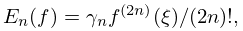
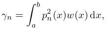
The are also known as Christoffel coefficients or Christoffel numbers and they are all positive. The remainder is given by
| 3.5.19 | |||
where
| 3.5.20 | |||
and is some point in . As a consequence, the rule is exact for any polynomial of degree , that is,
| 3.5.20_1 | |||
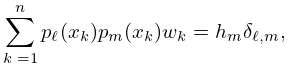
In particular, with , we have a finite system of orthogonal polynomials () on with respect to the weights :
| 3.5.20_2 | |||
| for . | |||
In practical applications the weight function is chosen to simulate the asymptotic behavior of the integrand as the endpoints are approached. For functions Gauss quadrature can be very efficient. In adaptive algorithms the evaluation of the nodes and weights may cause difficulties, unless exact values are known.
For the derivation of Gauss quadrature formulas see Gautschi (2004, pp. 22–32), Gil et al. (2007a, §5.3), and Davis and Rabinowitz (1984, §§2.7 and 3.6). Stroud and Secrest (1966) includes computational methods and extensive tables. For further extensions, applications, and computation of orthogonal polynomials and Gauss-type formulas, see Gautschi (1994, 1996, 2004). For effective testing of Gaussian quadrature rules see Gautschi (1983).
For the classical orthogonal polynomials related to the following Gauss rules, see §18.3. The given quantities follow from (18.2.5), (18.2.7), Table 18.3.1, and the relation .
Gauss–Legendre Formula
| 3.5.21 | ||||
The nodes and weights for , are shown in Tables 3.5.1 and 3.5.2. The are the monic Legendre polynomials, that is, the polynomials (§18.3) scaled so that the coefficient of the highest power of in their explicit forms is unity.
| 0.14887 43389 81631 211 | 0.29552 42247 14752 870 |
| 0.43339 53941 29247 191 | 0.26926 67193 09996 355 |
| 0.67940 95682 99024 406 | 0.21908 63625 15982 044 |
| 0.86506 33666 88984 511 | 0.14945 13491 50580 593 |
| 0.97390 65285 17171 720 | 0.06667 13443 08688 138 |
| 0.07652 65211 33497 33375 5 | 0.15275 33871 30725 85069 8 |
| 0.22778 58511 41645 07808 0 | 0.14917 29864 72603 74678 8 |
| 0.37370 60887 15419 56067 3 | 0.14209 61093 18382 05132 9 |
| 0.51086 70019 50827 09800 4 | 0.13168 86384 49176 62689 8 |
| 0.63605 36807 26515 02545 3 | 0.11819 45319 61518 41731 2 |
| 0.74633 19064 60150 79261 4 | 0.10193 01198 17240 43503 7 |
| 0.83911 69718 22218 82339 5 | 0.08327 67415 76704 74872 5 |
| 0.91223 44282 51325 90586 8 | 0.06267 20483 34109 06357 0 |
| 0.96397 19272 77913 79126 8 | 0.04060 14298 00386 94133 1 |
| 0.99312 85991 85094 92478 6 | 0.01761 40071 39152 11831 2 |
| 0.03877 24175 06050 82193 3 | 0.07750 59479 78424 81126 4 |
| 0.11608 40706 75255 20848 3 | 0.07703 98181 64247 96558 8 |
| 0.19269 75807 01371 09971 6 | 0.07611 03619 00626 24237 2 |
| 0.26815 21850 07253 68114 1 | 0.07472 31690 57968 26420 0 |
| 0.34199 40908 25758 47300 7 | 0.07288 65823 95804 05906 1 |
| 0.41377 92043 71605 00152 5 | 0.07061 16473 91286 77969 6 |
| 0.48307 58016 86178 71290 9 | 0.06791 20458 15233 90382 6 |
| 0.54946 71250 95128 20207 6 | 0.06480 40134 56601 03807 5 |
| 0.61255 38896 67980 23795 3 | 0.06130 62424 92928 93916 7 |
| 0.67195 66846 14179 54837 9 | 0.05743 97690 99391 55136 7 |
| 0.72731 82551 89927 10328 1 | 0.05322 78469 83936 82435 5 |
| 0.77830 56514 26519 38769 5 | 0.04869 58076 35072 23206 1 |
| 0.82461 22308 33311 66319 6 | 0.04387 09081 85673 27199 2 |
| 0.86595 95032 12259 50382 1 | 0.03878 21679 74472 01764 0 |
| 0.90209 88069 68874 29672 8 | 0.03346 01952 82547 84739 3 |
| 0.93281 28082 78676 53336 1 | 0.02793 70069 80023 40109 9 |
| 0.95791 68192 13791 65580 5 | 0.02224 58491 94166 95726 2 |
| 0.97725 99499 83774 26266 3 | 0.01642 10583 81907 88871 3 |
| 0.99072 62386 99457 00645 3 | 0.01049 82845 31152 81361 5 |
| 0.99823 77097 10559 20035 0 | 0.00452 12770 98533 19125 8 |
| 0.01951 13832 56793 99765 4 | 0.03901 78136 56306 65481 1 |
| 0.05850 44371 52420 66862 9 | 0.03895 83959 62769 53119 9 |
| 0.09740 83984 41584 59906 3 | 0.03883 96510 59051 96893 2 |
| 0.13616 40228 09143 88655 9 | 0.03866 17597 74076 46332 7 |
| 0.17471 22918 32646 81255 9 | 0.03842 49930 06959 42318 5 |
| 0.21299 45028 57666 13257 2 | 0.03812 97113 14477 63834 4 |
| 0.25095 23583 92272 12049 3 | 0.03777 63643 62001 39749 0 |
| 0.28852 80548 84511 85310 9 | 0.03736 54902 38730 49002 7 |
| 0.32566 43707 47701 91461 9 | 0.03689 77146 38276 00883 9 |
| 0.36230 47534 99487 31561 9 | 0.03637 37499 05835 97804 4 |
| 0.39839 34058 81969 22702 4 | 0.03579 43939 53416 05460 3 |
| 0.43387 53708 31756 09306 2 | 0.03516 05290 44747 59349 6 |
| 0.46869 66151 70544 47703 6 | 0.03447 31204 51753 92879 4 |
| 0.50280 41118 88784 98759 4 | 0.03373 32149 84611 52281 7 |
| 0.53614 59208 97131 93202 0 | 0.03294 19393 97645 40138 3 |
| 0.56867 12681 22709 78472 5 | 0.03210 04986 73487 77314 8 |
| 0.60033 06228 29751 74315 5 | 0.03121 01741 88114 70164 2 |
| 0.63107 57730 46871 96624 8 | 0.03027 23217 59557 98066 1 |
| 0.66085 98989 86119 80173 6 | 0.02928 83695 83267 84769 3 |
| 0.68963 76443 42027 60077 1 | 0.02825 98160 57276 86239 7 |
| 0.71736 51853 62099 88025 4 | 0.02718 82275 00486 38067 4 |
| 0.74400 02975 83597 27231 7 | 0.02607 52357 67565 11790 3 |
| 0.76950 24201 35041 37386 6 | 0.02492 25357 64115 49110 5 |
| 0.79383 27175 04605 44994 9 | 0.02373 18828 65930 10129 3 |
| 0.81695 41386 81463 47037 1 | 0.02250 50902 46332 46192 6 |
| 0.83883 14735 80255 27561 7 | 0.02124 40261 15782 00638 9 |
| 0.85943 14066 63111 09697 7 | 0.01995 06108 78141 99892 9 |
| 0.87872 25676 78213 82870 4 | 0.01862 68142 08299 03142 9 |
| 0.89667 55794 38770 68319 4 | 0.01727 46520 56269 30635 9 |
| 0.91326 31025 71757 65416 5 | 0.01589 61835 83725 68804 5 |
| 0.92845 98771 72445 79595 3 | 0.01449 35080 40509 07611 7 |
| 0.94224 27613 09872 67475 2 | 0.01306 87615 92401 33929 4 |
| 0.95459 07663 43634 90549 3 | 0.01162 41141 20797 82691 7 |
| 0.96548 50890 43799 25145 2 | 0.01016 17660 41103 06452 1 |
| 0.97490 91405 85727 79338 6 | 0.00868 39452 69260 85842 6 |
| 0.98284 85727 38629 07041 8 | 0.00719 29047 68117 31275 3 |
| 0.98929 13024 99755 53102 7 | 0.00569 09224 51403 19864 9 |
| 0.99422 75409 65688 27789 2 | 0.00418 03131 24694 89523 7 |
| 0.99764 98643 98237 68889 9 | 0.00266 35335 89512 68166 9 |
| 0.99955 38226 51630 62988 0 | 0.00114 49500 03186 94153 5 |
Gauss–Chebyshev Formula
| 3.5.22 | ||||
The nodes and weights are known explicitly:
| 3.5.23 | ||||
| , | ||||
| . | ||||
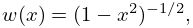
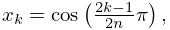
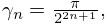
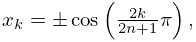
In the case of Chebyshev weight functions on , with , the nodes , weights , and error constant , are as follows:
| 3.5.24 | ||||
| , | ||||
and
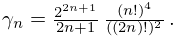
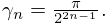
| 3.5.25 | ||||
| , | ||||
where .
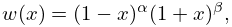
Gauss–Jacobi Formula
| 3.5.26 | ||||
| , . | ||||
The are the monic Jacobi polynomials (§18.3).
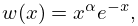
Gauss–Laguerre Formula
| 3.5.27 | ||||
| . | ||||
If this is called the generalized Gauss–Laguerre formula.
The nodes and weights for and , are shown in Tables 3.5.6 and 3.5.7. The are the monic Laguerre polynomials (§18.3).
Gauss–Hermite Formula
| 3.5.28 | ||||
The nodes and weights for are shown in Tables 3.5.10 and 3.5.11. The are the monic Hermite polynomials (§18.3).
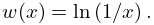
Gauss Formula for a Logarithmic Weight Function
| 3.5.29 | ||||
§3.5(vi) Eigenvalue/Eigenvector Characterization of Gauss Quadrature Formulas
All the monic orthogonal polynomials used with Gauss quadrature satisfy a three-term recurrence relation (§18.2(iv)):
| 3.5.30 | |||
| , | |||
with , , and . Then . The corresponding orthonormal polynomials satisfy the recurrence relation
| 3.5.30_5 | |||
| , | |||
with , and .
The monic and orthonormal recursion relations of this section are both closely related to the Lanczos recursion relation in §3.2(vi).
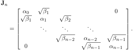
The Gauss nodes (the zeros of ) are the eigenvalues of the (symmetric tridiagonal) Jacobi matrix of order :
| 3.5.31 | |||
Let denote the normalized eigenvector of corresponding to the eigenvalue . Then the weights are given by
| 3.5.32 | |||
| , | |||
where and is the first element of . Also, the error constant (3.5.20) is given by
| 3.5.33 | |||
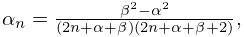
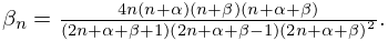
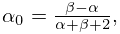
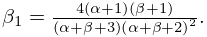
Tables 3.5.1–3.5.13 can be verified by application of the results given in the present subsection. The monic version and orthonormal version of a classical orthogonal polynomial are obtained by dividing the orthogonal polynomial by respectively , with and as in Table 18.3.1. Below we give for the classical orthogonal polynomials the recurrence coefficients and in (3.5.30). These also immediately yield the recurrence coefficients in (3.5.30_5). In case of the Jacobi polynomials we have , , and
| 3.5.33_1 | ||||
In particular, by continuity in and ,
| 3.5.33_2 | ||||
Furthermore, . For the other classical OP’s see Table 3.5.17_5.
§3.5(vii) Oscillatory Integrals
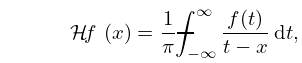
Integrals of the form
| 3.5.34 | |||
can be computed by Filon’s rule. See Davis and Rabinowitz (1984, pp. 146–168).
Oscillatory integral transforms are treated in Wong (1982) by a method based on Gaussian quadrature. A comparison of several methods, including an extension of the Clenshaw–Curtis formula (§3.5(iv)), is given in Evans and Webster (1999).
For computing infinite oscillatory integrals, Longman’s method may be used. The integral is written as an alternating series of positive and negative subintegrals that are computed individually; see Longman (1956). Convergence acceleration schemes, for example Levin’s transformation (§3.9(v)), can be used when evaluating the series. Further methods are given in Clendenin (1966) and Lyness (1985).
For a comprehensive survey of quadrature of highly oscillatory integrals, including multidimensional integrals, see Iserles et al. (2006).
§3.5(viii) Complex Gauss Quadrature
For the Bromwich integral
| 3.5.35 | |||
| , , | |||
a complex Gauss quadrature formula is available. Here is assumed analytic in the half-plane and bounded as in . The quadrature rule for (3.5.35) is
| 3.5.36 | |||
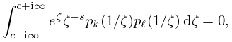
where if is a polynomial of degree in . Complex orthogonal polynomials of degree , in that satisfy the orthogonality condition
| 3.5.37 | |||
| , | |||
are related to Bessel polynomials (§§10.49(ii) and 18.34). The complex Gauss nodes have positive real part for all .
The nodes and weights of the 5-point complex Gauss quadrature formula (3.5.36) for are shown in Table 3.5.18. Extensive tables of quadrature nodes and weights can be found in Krylov and Skoblya (1985).
Example. Laplace Transform Inversion
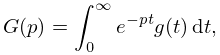
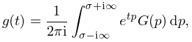
From §1.14(iii)
| 3.5.38 | |||
| 3.5.39 | |||
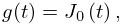
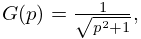
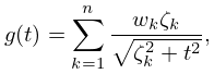
with appropriate conditions. The pair
| 3.5.40 | ||||
where is the Bessel function (§10.2(ii)), satisfy these conditions, provided that . The integral (3.5.39) has the form (3.5.35) if we set , , and . We choose so that at infinity. Equation (3.5.36), without the error term, becomes
| 3.5.41 | |||
approximately.
Using Table 3.5.18 we compute for . The results are given in the middle column of Table 3.5.19, accompanied by the actual 10D values in the last column. Agreement is very good for small values of , but not for larger values. For these cases the integration path may need to be deformed; see §3.5(ix).
| 0.0 | 1.00000 00000 | 1.00000 00000 |
|---|---|---|
| 0.5 | 0.93846 98072 | 0.93846 98072 |
| 1.0 | 0.76519 76866 | 0.76519 76865 |
| 2.0 | 0.22389 07791 | 0.22389 10326 |
| 5.0 | 0.17759 67713 | 0.17902 54097 |
| 10.0 | 0.24593 57645 | 0.07540 53543 |
§3.5(ix) Other Contour Integrals
A frequent problem with contour integrals is heavy cancellation, which occurs especially when the value of the integral is exponentially small compared with the maximum absolute value of the integrand. To avoid cancellation we try to deform the path to pass through a saddle point in such a way that the maximum contribution of the integrand is derived from the neighborhood of the saddle point. For example, steepest descent paths can be used; see §2.4(iv).
Example
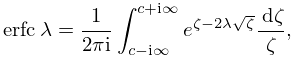
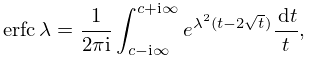
In (3.5.35) take and , with . When is large the integral becomes exponentially small, and application of the quadrature rule of §3.5(viii) is useless. In fact from (7.14.4) and the inversion formula for the Laplace transform (§1.14(iii)) we have
| 3.5.42 | |||
| , | |||
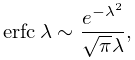
where is the complementary error function, and from (7.12.1) it follows that
| 3.5.43 | |||
| . | |||
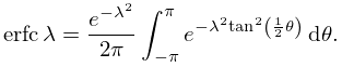
With the transformation , (3.5.42) becomes
| 3.5.44 | |||
| , | |||
with saddle point at , and when the vertical path intersects the real axis at the saddle point. The steepest descent path is given by , or in polar coordinates we have . Thus
| 3.5.45 | |||
The integrand can be extended as a periodic function on with period and as noted in §3.5(i), the trapezoidal rule is exceptionally efficient in this case.
Table 3.5.20 gives the results of applying the composite trapezoidal rule (3.5.2) with step size ; indicates the number of function values in the rule that are larger than (we exploit the fact that the integrand is even). All digits shown in the approximation in the final row are correct.
| 5 | ||||
| 6 | ||||
| 8 | ||||
| 11 | ||||
A second example is provided in Gil et al. (2001), where the method of contour integration is used to evaluate Scorer functions of complex argument (§9.12). See also Gil et al. (2003b).
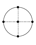
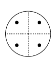
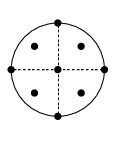
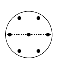
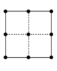
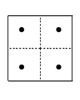
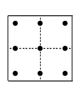
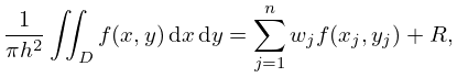
§3.5(x) Cubature Formulas
Table 3.5.21 supplies cubature rules, including weights , for the disk , given by :
| 3.5.47 | |||
and the square , given by , :
| 3.5.48 | |||
For these results and further information on cubature formulas see Cools (2003).
For integrals in higher dimensions, Monte Carlo methods are another—often the only—alternative. The standard Monte Carlo method samples points uniformly from the integration region to estimate the integral and its error. In more advanced methods points are sampled from a probability distribution, so that they are concentrated in regions that make the largest contribution to the integral. With function values, the Monte Carlo method aims at an error of order , independently of the dimension of the domain of integration. See Davis and Rabinowitz (1984, pp. 384–417) and Schürer (2004).
| Diagram | |||
|---|---|---|---|
|
|||
|
|||
|
|||
| , | |||
|
|||
|
|||
| , | |||
|
|||
|
|||
| , | |||
