Hermite polynomials

SearchAdvancedHelp

(0.007 seconds)

1—10 of 59 matching pages

1: 18.3 Definitions

§18.3 Definitions

►The classical OP’s comprise the Jacobi, Laguerre and Hermite polynomials. … ►Table 18.3.1 provides the traditional definitions of Jacobi, Laguerre, and Hermite polynomials via orthogonality and standardization (§§18.2(i) and 18.2(iii)). … ►

Table 18.3.1: Orthogonality properties for classical OP’s: intervals, weight functions, standardizations, leading coefficients, and parameter constraints. …

► ►►►►

Name	$p_n(x)$	$(a,b)$	$w(x)$	$h_n$	$k_n$	${\tilde{k}}_n/k_n$	Constraints
…
Hermite	$H_n\left(x\right)$	$(-\mathrm{\infty },\mathrm{\infty })$	${\mathrm{e}}^{-x^2}$	${\pi }^{\frac{1}{2}}{2}^{n}n!$	$2^n$	$0$
Hermite	${\mathrm{𝐻𝑒}}_n\left(x\right)$	$(-\mathrm{\infty },\mathrm{\infty })$	${\mathrm{e}}^{-\frac{1}{2}{x}^2}$	${(2\pi )}^{\frac{1}{2}}n!$	$1$	$0$

►

…

2: 18.41 Tables

… ►For $P_n\left(x\right)$ ($={𝖯}_n\left(x\right)$) see §14.33. ►Abramowitz and Stegun (1964, Tables 22.4, 22.6, 22.11, and 22.13) tabulates $T_n\left(x\right)$, $U_n\left(x\right)$, $L_n\left(x\right)$, and $H_n\left(x\right)$ for $n=0(1)12$. The ranges of $x$ are $0.2(.2)1$ for $T_n\left(x\right)$ and $U_n\left(x\right)$, and $0.5,1,3,5,10$ for $L_n\left(x\right)$ and $H_n\left(x\right)$. The precision is 10D, except for $H_n\left(x\right)$ which is 6-11S. … ►For $P_n\left(x\right)$, $L_n\left(x\right)$, and $H_n\left(x\right)$ see §3.5(v). …

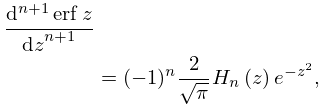
3: 7.10 Derivatives

§7.10 Derivatives

►

7.10.1 $$\frac{d^{n+1}\mathrm{erf}z}{{dz}^{n+1}}={(-1)}^n\frac{2}{\sqrt{\pi }}{H}_n\left(z\right){\mathrm{e}}^{-z^2},$$ $n=0,1,2,\mathrm{\dots }$.

ⓘ

Symbols:

$H_n\left(x\right)$: Hermite polynomial, $\pi$: the ratio of the circumference of a circle to its diameter, $\frac{df}{dx}$: derivative of $f$ with respect to $x$ , $\mathrm{erf}z$: error function, $\mathrm{e}$: base of natural logarithm, $z$: complex variable and $n$: nonnegative integer

A&S Ref:

7.1.19

Permalink:

http://dlmf.nist.gov/7.10.E1

Encodings:

pMML, png, TeX

See also:

Annotations for §7.10 and Ch.7

►For the Hermite polynomial $H_n\left(z\right)$ see §18.3. …

4: 18.36 Miscellaneous Polynomials

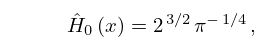
… ►The type III $X_2$-Hermite EOP’s, missing polynomial orders $1$ and $2$, are the complete set of polynomials, with real coefficients and defined explicitly as ►

18.36.8 $${\widehat{H}}_0\left(x\right)=2^{3/2}{\pi }^{-1/4},$$

ⓘ

Symbols:

$\pi$: the ratio of the circumference of a circle to its diameter, ${\widehat{H}}_n\left(x\right)$: exceptional Hermite polynomial and $x$: real variable

Referenced by:

§18.39(i)

Permalink:

http://dlmf.nist.gov/18.36.E8

Encodings:

pMML, png, TeX

See also:

Annotations for §18.36(vi), §18.36(vi), §18.36 and Ch.18

►

18.36.9 $${\widehat{H}}_{n+3}\left(x\right)=\frac{(4x^2+2)H_{n+1}\left(x\right)+8x{H}_n\left(x\right)}{{\pi }^{1/4}\sqrt{2^{n+1}(n+3)n!}}=\frac{𝒲\left\{H_1\left(x\right),H_2\left(x\right),H_{n+3}\left(x\right)\right\}}{{\pi }^{1/4}\sqrt{2^{n+7}(n+1)(n+2)(n+3)!}},$$ $n=0,1,\mathrm{\dots }$,

ⓘ

Symbols:

$H_n\left(x\right)$: Hermite polynomial, $𝒲$: Wronskian, $\pi$: the ratio of the circumference of a circle to its diameter, ${\widehat{H}}_n\left(x\right)$: exceptional Hermite polynomial, $!$: factorial (as in $n!$), $n$: nonnegative integer and $x$: real variable

Referenced by:

§18.39(i)

Permalink:

http://dlmf.nist.gov/18.36.E9

Encodings:

pMML, png, TeX

Addition (effective with 1.2.0):

This equation was added.

See also:

Annotations for §18.36(vi), §18.36(vi), §18.36 and Ch.18

… ►In §18.39(i) it is seen that the functions, $\sqrt{w(x)}{\widehat{H}}_{n+3}\left(x\right)$, are solutions of a Schrödinger equation with a rational potential energy; and, in spite of first appearances, the Sturm oscillation theorem, Simon (2005c, Theorem 3.3, p. 35), is satisfied. …

5: 28.9 Zeros

… ►For $q\to \mathrm{\infty }$ the zeros of ${\mathrm{ce}}_{2n}(z,q)$ and ${\mathrm{se}}_{2n+1}(z,q)$ approach asymptotically the zeros of ${\mathrm{𝐻𝑒}}_{2n}\left(q^{1/4}(\pi -2z)\right)$, and the zeros of ${\mathrm{ce}}_{2n+1}(z,q)$ and ${\mathrm{se}}_{2n+2}(z,q)$ approach asymptotically the zeros of ${\mathrm{𝐻𝑒}}_{2n+1}\left(q^{1/4}(\pi -2z)\right)$. Here ${\mathrm{𝐻𝑒}}_n\left(z\right)$ denotes the Hermite polynomial of degree $n$ (§18.3). …

6: 18.8 Differential Equations

… ►

Table 18.8.1: Classical OP’s: differential equations $A(x)f^{\prime \prime }(x)+B(x)f^{\prime }(x)+C(x)f(x)+{\lambda }_{n}f(x)=0$.

► ►►►►►

#	$f(x)$	$A(x)$	$B(x)$	$C(x)$	${\lambda }_n$
…
12	$H_n\left(x\right)$	$1$	$-2x$	$0$	$2n$
13	${\mathrm{e}}^{-\frac{1}{2}{x}^2}{H}_n\left(x\right)$	$1$	$0$	$-x^2$	$2n+1$
14	${\mathrm{𝐻𝑒}}_n\left(x\right)$	$1$	$-x$	$0$	$n$

►

…

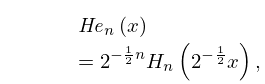
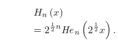
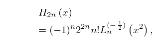
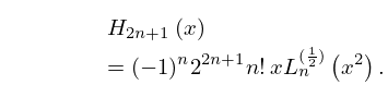
7: 18.7 Interrelations and Limit Relations

§18.7 Interrelations and Limit Relations

… ►

18.7.11 $${\mathrm{𝐻𝑒}}_n\left(x\right)=2^{-\frac{1}{2}n}{H}_n\left(2^{-\frac{1}{2}}x\right),$$

ⓘ

Symbols:

$H_n\left(x\right)$: Hermite polynomial, ${\mathrm{𝐻𝑒}}_n\left(x\right)$: Hermite polynomial, $n$: nonnegative integer and $x$: real variable

A&S Ref:

22.5.18

Referenced by:

§18.5(iii)

Permalink:

http://dlmf.nist.gov/18.7.E11

Encodings:

pMML, png, TeX

See also:

Annotations for §18.7(i), §18.7(i), §18.7 and Ch.18

►

18.7.12 $$H_n\left(x\right)=2^{\frac{1}{2}n}{\mathrm{𝐻𝑒}}_n\left(2^{\frac{1}{2}}x\right).$$

ⓘ

Symbols:

$H_n\left(x\right)$: Hermite polynomial, ${\mathrm{𝐻𝑒}}_n\left(x\right)$: Hermite polynomial, $n$: nonnegative integer and $x$: real variable

A&S Ref:

22.5.19

Referenced by:

§18.7(i)

Permalink:

http://dlmf.nist.gov/18.7.E12

Encodings:

pMML, png, TeX

See also:

Annotations for §18.7(i), §18.7(i), §18.7 and Ch.18

… ►

18.7.19 $$H_{2n}\left(x\right)={(-1)}^n{2}^{2n}n!L_n^{(-\frac{1}{2})}\left(x^2\right),$$

ⓘ

Symbols:

$H_n\left(x\right)$: Hermite polynomial, $L_n^{(\alpha )}\left(x\right)$: Laguerre (or generalized Laguerre) polynomial, $!$: factorial (as in $n!$), $n$: nonnegative integer and $x$: real variable

A&S Ref:

22.5.40

Referenced by:

§18.16(v), §18.18(iii), §18.18(iv), §18.18(viii), §18.7(ii)

Permalink:

http://dlmf.nist.gov/18.7.E19

Encodings:

pMML, png, TeX

See also:

Annotations for §18.7(ii), §18.7 and Ch.18

►

18.7.20 $$H_{2n+1}\left(x\right)={(-1)}^n{2}^{2n+1}n!x{L}_n^{(\frac{1}{2})}\left(x^2\right).$$

ⓘ

Symbols:

$H_n\left(x\right)$: Hermite polynomial, $L_n^{(\alpha )}\left(x\right)$: Laguerre (or generalized Laguerre) polynomial, $!$: factorial (as in $n!$), $n$: nonnegative integer and $x$: real variable

A&S Ref:

22.5.41

Referenced by:

§18.16(v), §18.18(iii), §18.18(iv), §18.7(ii), §18.7(ii)

Permalink:

http://dlmf.nist.gov/18.7.E20

Encodings:

pMML, png, TeX

See also:

Annotations for §18.7(ii), §18.7 and Ch.18

…

8: 18.6 Symmetry, Special Values, and Limits to Monomials

… ►For Jacobi, ultraspherical, Chebyshev, Legendre, and Hermite polynomials, see Table 18.6.1. … ►

Table 18.6.1: Classical OP’s: symmetry and special values.

► ►►►►

$p_n(x)$	$p_n(-x)$	$p_n(1)$	$p_{2n}(0)$	$p_{2n+1}^{\prime }(0)$
…
$H_n\left(x\right)$	${(-1)}^n{H}_n\left(x\right)$		${(-1)}^n{\left(n+1\right)}_n$	$2{(-1)}^n{\left(n+1\right)}_{n+1}$
${\mathrm{𝐻𝑒}}_n\left(x\right)$	${(-1)}^n{\mathrm{𝐻𝑒}}_n\left(x\right)$		${(-\frac{1}{2})}^n{\left(n+1\right)}_n$	${(-\frac{1}{2})}^n{\left(n+1\right)}_{n+1}$

►

…

9: 18.17 Integrals

… ►

Hermite

… ►

Hermite

… ►

Hermite

… ►

Hermite

… ►

Hermite

…

10: 12.7 Relations to Other Functions

… ►

§12.7(i) Hermite Polynomials

… ►

12.7.2 $$U(-n-\frac{1}{2},z)=D_n\left(z\right)={\mathrm{e}}^{-\frac{1}{4}{z}^2}{\mathrm{𝐻𝑒}}_n\left(z\right)=2^{-n/2}{\mathrm{e}}^{-\frac{1}{4}{z}^2}{H}_n\left(z/\sqrt{2}\right),$$ $n=0,1,2,\mathrm{\dots }$ ,

ⓘ

Symbols:

$H_n\left(x\right)$: Hermite polynomial, ${\mathrm{𝐻𝑒}}_n\left(x\right)$: Hermite polynomial, $D_{\nu }\left(z\right)$: parabolic cylinder function, $\mathrm{e}$: base of natural logarithm, $U(a,z)$: parabolic cylinder function, $z$: complex variable and $n$: nonnegative integer

A&S Ref:

19.13.1 (modification of)

Permalink:

http://dlmf.nist.gov/12.7.E2

Encodings:

pMML, png, TeX

See also:

Annotations for §12.7(i), §12.7 and Ch.12

►

12.7.3 $$V(n+\frac{1}{2},z)=\sqrt{2/\pi }{\mathrm{e}}^{\frac{1}{4}{z}^2}{(-\mathrm{i})}^n{\mathrm{𝐻𝑒}}_n\left(\mathrm{i}z\right)=\sqrt{2/\pi }{\mathrm{e}}^{\frac{1}{4}{z}^2}{(-\mathrm{i})}^n{2}^{-\frac{1}{2}n}{H}_n\left(\mathrm{i}z/\sqrt{2}\right),$$ $n=0,1,2,\mathrm{\dots }$.

ⓘ

Symbols:

$H_n\left(x\right)$: Hermite polynomial, ${\mathrm{𝐻𝑒}}_n\left(x\right)$: Hermite polynomial, $\pi$: the ratio of the circumference of a circle to its diameter, $\mathrm{e}$: base of natural logarithm, $\mathrm{i}$: imaginary unit, $V(a,z)$: parabolic cylinder function, $z$: complex variable and $n$: nonnegative integer

A&S Ref:

19.13.2 (corrected)

Permalink:

http://dlmf.nist.gov/12.7.E3

Encodings:

pMML, png, TeX

See also:

Annotations for §12.7(i), §12.7 and Ch.12

…