§6.18 Methods of Computation

For small or moderate values of and , the expansion in power series (§6.6) or in series of spherical Bessel functions (§6.10(ii)) can be used. For large or these series suffer from slow convergence or cancellation (or both). However, this problem is less severe for the series of spherical Bessel functions because of their more rapid rate of convergence, and also (except in the case of (6.10.6)) absence of cancellation when ().

For large and , expansions in inverse factorial series (§6.10(i)) or asymptotic expansions (§6.12) are available. The attainable accuracy of the asymptotic expansions can be increased considerably by exponential improvement. Also, other ranges of can be covered by use of the continuation formulas of §6.4.

Quadrature of the integral representations is another effective method. For example, the Gauss-Laguerre formula (§3.5(v)) can be applied to (6.2.2); see Todd (1954) and Tseng and Lee (1998). For an application of the Gauss-Legendre formula (§3.5(v)) see Tooper and Mark (1968).

Lastly, the continued fraction (6.9.1) can be used if is bounded away from the origin. Convergence becomes slow when is near the negative real axis, however.

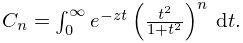
Power series, asymptotic expansions, and quadrature can also be used to compute the functions and . In addition, Acton (1974) developed a recurrence procedure, as follows. For , define

6.18.1

Symbols:

: differential of , : base of exponential function, : integral, : complex variable and : nonnegative integer

Permalink:

http://dlmf.nist.gov/6.18.E1

Encodings:

TeX, TeX, TeX, pMML, pMML, pMML, png, png, png

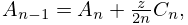
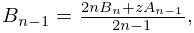
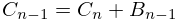
Then , , and

6.18.2

,

Symbols:

: complex variable and : nonnegative integer

Permalink:

http://dlmf.nist.gov/6.18.E2

Encodings:

TeX, TeX, TeX, pMML, pMML, pMML, png, png, png

, , and can be computed by Miller’s algorithm (§3.6(iii)), starting with initial values , say, where is an arbitrary large integer, and normalizing via .

Zeros of and can be computed to high precision by Newton’s rule (§3.8(ii)), using values supplied by the asymptotic expansion (6.13.2) as initial approximations.

For a comprehensive survey of computational methods for the functions treated in this chapter, see van der Laan and Temme (1984, Ch. IV).