§1.14 Integral Transforms
Contents
- §1.14(i) Fourier Transform
- §1.14(ii) Fourier Cosine and Sine Transforms
- §1.14(iii) Laplace Transform
- §1.14(iv) Mellin Transform
- §1.14(v) Hilbert Transform
- §1.14(vi) Stieltjes Transform
- §1.14(vii) Tables
- §1.14(viii) Compendia
§1.14(i) Fourier Transform
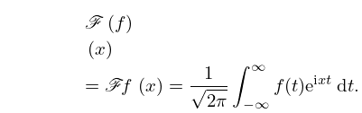
The Fourier transform of a real- or complex-valued function is defined by
| 1.14.1 | |||
(Some references replace by ). The same notation is used for Fourier transforms of functions of several variables and for Fourier transforms of distributions; see §1.16(vii).
In this subsection we let .
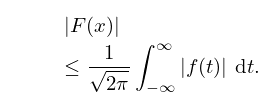
If is absolutely integrable on , then is continuous, as , and
| 1.14.2 | |||
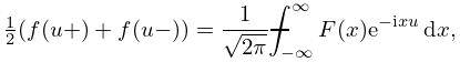
Inversion
Suppose that is absolutely integrable on and of bounded variation in a neighborhood of (§1.4(v)). Then
| 1.14.3 | |||
where the last integral denotes the Cauchy principal value (1.4.25).
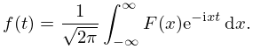
In many applications is absolutely integrable and is continuous on . Then
| 1.14.4 | |||
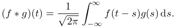
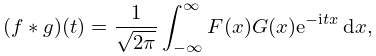
Convolution
For Fourier transforms, the convolution of two functions and defined on is given by
| 1.14.5 | |||
If and are absolutely integrable on , then so is , and its Fourier transform is , where is the Fourier transform of .
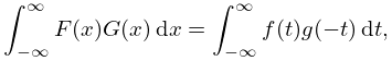
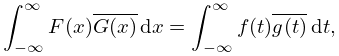
Parseval’s Formula
Poisson’s Summation Formula
Uniqueness
If and are continuous and absolutely integrable on , and for all , then for all .
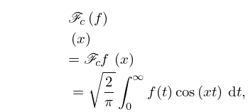
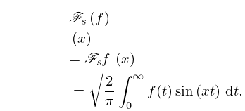
§1.14(ii) Fourier Cosine and Sine Transforms
The Fourier cosine transform and Fourier sine transform are defined respectively by
| 1.14.9 | ||||
| 1.14.10 | ||||
In this subsection we let , , , and .
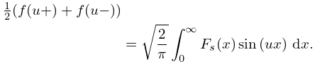
Inversion
If is absolutely integrable on and of bounded variation (§1.4(v)) in a neighborhood of , then
| 1.14.11 | ||||
| 1.14.12 | ||||
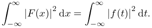
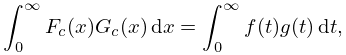
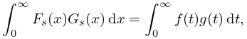
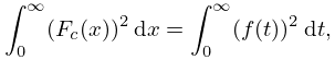
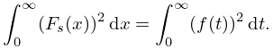
Parseval’s Formula
Suppose and are absolutely and square integrable on , then
| 1.14.13 | ||||
| 1.14.14 | ||||
| 1.14.15 | ||||
| 1.14.16 | ||||
§1.14(iii) Laplace Transform
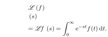
Suppose is a real- or complex-valued function and is a real or complex parameter. The Laplace transform of is defined by
| 1.14.17 | |||
Convergence and Analyticity
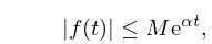
Assume that is piecewise continuous on and of exponential growth, that is, constants and exist such that
| 1.14.18 | |||
| . | |||
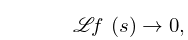
Then is an analytic function of for . Moreover,
| 1.14.19 | |||
| . | |||
Throughout the remainder of this subsection we assume (1.14.18) is satisfied and .
Inversion
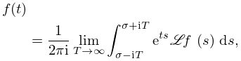
If is continuous and is piecewise continuous on , then
| 1.14.20 | |||
| . | |||
Moreover, if in some half-plane and , then (1.14.20) holds for .
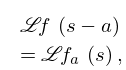
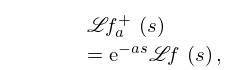
Translation
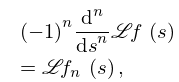
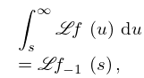
Differentiation and Integration
If is piecewise continuous, then
| 1.14.23 | |||
| , | |||
where . If also exists, then
| 1.14.24 | |||
where .
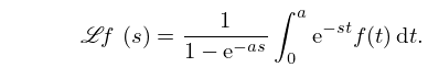
Periodic Functions
If and for , then
| 1.14.25 | |||
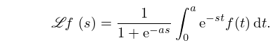
Alternatively if for , then
| 1.14.26 | |||
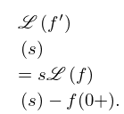
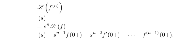
Derivatives
If is continuous on and is piecewise continuous on , then
| 1.14.27 | |||
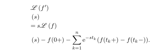
If and are piecewise continuous on with discontinuities at () , then
| 1.14.28 | |||
Next, assume , , , are continuous and each satisfies (1.14.18). Also assume that is piecewise continuous on . Then
| 1.14.29 | |||
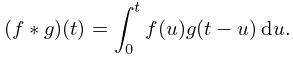
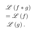
Convolution
For Laplace transforms, the convolution of two functions and , defined on , is
| 1.14.30 | |||
If and are piecewise continuous, then
| 1.14.31 | |||
Uniqueness
If and are continuous and , then .
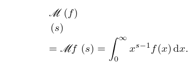
§1.14(iv) Mellin Transform
The Mellin transform of a real- or complex-valued function is defined by
| 1.14.32 | |||
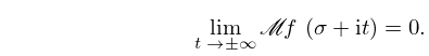
If is integrable on for all in , then the integral (1.14.32) converges and is an analytic function of in the vertical strip . Moreover, for ,
| 1.14.33 | |||
Note: If is continuous and and are real numbers such that as and as , then is integrable on for all .
Inversion
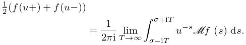
Suppose the integral (1.14.32) is absolutely convergent on the line and is of bounded variation in a neighborhood of . Then
| 1.14.34 | |||
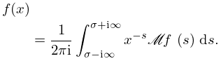
If is continuous on and is integrable on , then
| 1.14.35 | |||
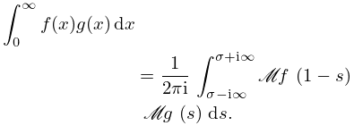
Parseval-type Formulas
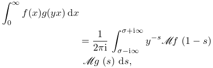
Suppose and are absolutely integrable on and either or is absolutely integrable on . Then for ,
| 1.14.36 | |||
| 1.14.37 | |||
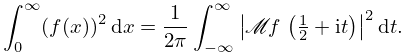
When is real and ,
| 1.14.38 | |||
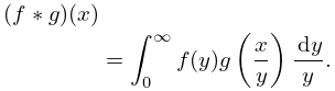
Convolution
Let
| 1.14.39 | |||
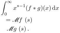
If and are absolutely integrable on , then for ,
| 1.14.40 | |||
§1.14(v) Hilbert Transform
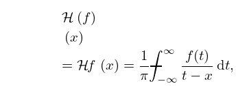
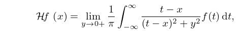
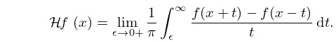
The Hilbert transform of a real-valued function is defined in the following equivalent ways:
| 1.14.41 | ||||
| 1.14.42 | ||||
| 1.14.43 | ||||
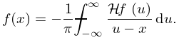
Inversion
Suppose is continuously differentiable on and vanishes outside a bounded interval. Then
| 1.14.44 | |||
Inequalities
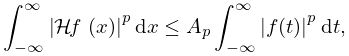
If , , is integrable on , then so is and
| 1.14.45 | |||
where when , or when . These bounds are sharp, and equality holds when .
Fourier Transform
§1.14(vi) Stieltjes Transform
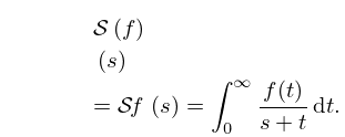
The Stieltjes transform of a real-valued function is defined by
| 1.14.47 | |||
Sufficient conditions for the integral to converge are that is a positive real number, and as , where .
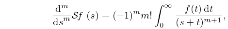
If the integral converges, then it converges uniformly in any compact domain in the complex -plane not containing any point of the interval . In this case, represents an analytic function in the -plane cut along the negative real axis, and
| 1.14.48 | |||
| . | |||
Inversion
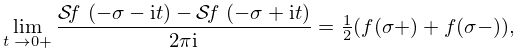
If is absolutely integrable on for every finite , and the integral (1.14.47) converges, then
| 1.14.49 | |||
for all values of the positive constant for which the right-hand side exists.
Laplace Transform
If is piecewise continuous on and the integral (1.14.47) converges, then
| 1.14.50 | |||
§1.14(vii) Tables
| , | ||
| , | ||
| , | ||
| , | ||
| , | ||
| , | ||
| , | ||
| , | ||
| , |
| , | ||
|---|---|---|
| , | ||
| , | ||
| , | ||
| , | ||
| , | ||
| , | ||
| , | ||
| , | ||
| , | , |
| , | ||
|---|---|---|
| , | ||
| , | ||
| , | ||
| , | ||
| , | ||
| , | ||
| , | ||
| , | ||
| , | ||
| , |
| , | ||
| , | ||
| , | ||
| , | ||
| , | ||
| , | , , | |
| , | ||
| , | ||
| , | ||
| , | ||
| , | ||
| , | ||
| , | , | |
| , | ||
| , | ||
| , |
| , | , | |
| , | , | |
| , | , (Cauchy p. v.) | |
| , | ||
| , | , | |
| , | ||
| , | ||
| , | ||
| , | ||
| , | , | |
| , | , |
§1.14(viii) Compendia
For more extensive tables of the integral transforms of this section and tables of other integral transforms, see Erdélyi et al. (1954a, b), Gradshteyn and Ryzhik (2000), Marichev (1983), Oberhettinger (1972, 1974, 1990), Oberhettinger and Badii (1973), Oberhettinger and Higgins (1961), Prudnikov et al. (1986a, b, 1990, 1992a, 1992b).
