§2.10 Sums and Sequences
Contents
- §2.10(i) Euler–Maclaurin Formula
- §2.10(ii) Summation by Parts
- §2.10(iii) Asymptotic Expansions of Entire Functions
- §2.10(iv) Taylor and Laurent Coefficients: Darboux’s Method
§2.10(i) Euler–Maclaurin Formula
As in §24.2, let and denote the th Bernoulli number and polynomial, respectively, and the th Bernoulli periodic function .
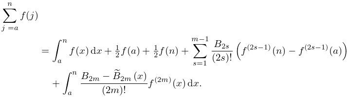
Assume that , and are integers such that , , and is absolutely integrable over . Then
| 2.10.1 | |||
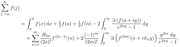
This is the Euler–Maclaurin formula. Another version is the Abel–Plana formula:
| 2.10.2 | |||
being some number in the interval . Sufficient conditions for the validity of this second result are:
-
(a)
On the strip , is analytic in its interior, is continuous on its closure, and as , uniformly with respect to .
-
(b)
is real when .
-
(c)
The first infinite integral in (2.10.2) converges.
Example
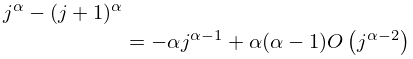
| 2.10.3 | |||
for large . From (2.10.1)
| 2.10.4 | |||
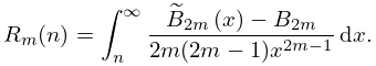
where () is arbitrary, is a constant, and
| 2.10.5 | |||
From §24.12(i), (24.2.2), and (24.4.27), is of constant sign . Thus and are of opposite signs, and since their difference is the term corresponding to in (2.10.4), is bounded in absolute value by this term and has the same sign.
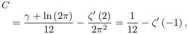
Formula (2.10.2) is useful for evaluating the constant term in expansions obtained from (2.10.1). In the present example it leads to
| 2.10.6 | |||
where is Euler’s constant (§5.2(ii)) and is the derivative of the Riemann zeta function (§25.2(i)). is sometimes called Glaisher’s constant. For further information on see §5.17.
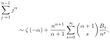
Other examples that can be verified in a similar way are:
| 2.10.7 | |||
| , | |||
where () is a real constant, and
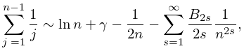
| 2.10.8 | |||
| . | |||
In both expansions the remainder term is bounded in absolute value by the first neglected term in the sum, and has the same sign, provided that in the case of (2.10.7), truncation takes place at , where is any positive integer satisfying .
For extensions of the Euler–Maclaurin formula to functions with singularities at or (or both) see Sidi (2004, 2012b, 2012a). See also Weniger (2007).
For an extension to integrals with Cauchy principal values see Elliott (1998).
§2.10(ii) Summation by Parts
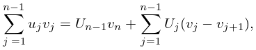
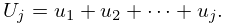
The formula for summation by parts is
| 2.10.9 | |||
where
| 2.10.10 | |||
This identity can be used to find asymptotic approximations for large when the factor changes slowly with , and is oscillatory; compare the approximation of Fourier integrals by integration by parts in §2.3(i).
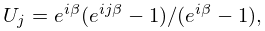
Example
| 2.10.11 | |||
where and are real constants with .
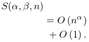
As a first estimate for large
| 2.10.12 | |||
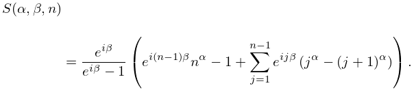
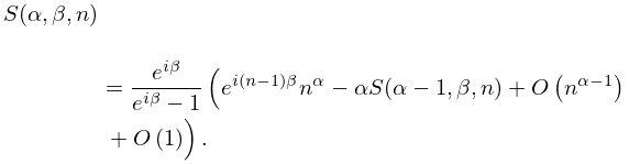
according as , , or see (2.10.7), (2.10.8). With , ,
| 2.10.13 | |||
and
| 2.10.14 | |||
Since
| 2.10.15 | |||
for any real constant and the set of all positive integers , we derive
| 2.10.16 | |||
From this result and (2.10.12)
| 2.10.17 | |||
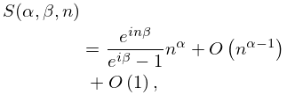
Then replacing by and resubstituting in (2.10.16), we have
| 2.10.18 | |||
| , | |||
which is a useful approximation when .
For extensions to , higher terms, and other examples, see Olver (1997b, Chapter 8).
§2.10(iii) Asymptotic Expansions of Entire Functions
The asymptotic behavior of entire functions defined by Maclaurin series can be approached by converting the sum into a contour integral by use of the residue theorem and applying the methods of §§2.4 and 2.5.
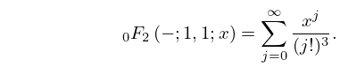
Example
| 2.10.19 | |||
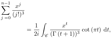
We seek the behavior as . From (1.10.8)
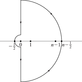
| 2.10.20 | |||
where comprises the two semicircles and two parts of the imaginary axis depicted in Figure 2.10.1.
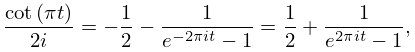
From the identities
| 2.10.21 | |||
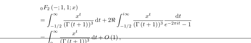
and Cauchy’s theorem, we have
| 2.10.22 | |||
where denote respectively the upper and lower halves of . (5.11.7) shows that the integrals around the large quarter circles vanish as . Hence
| 2.10.23 | |||
| , | |||
the last step following from when is on the interval , the imaginary axis, or the small semicircle. By application of Laplace’s method (§2.3(iii)) and use again of (5.11.7), we obtain
| 2.10.24 | |||
| . | |||
§2.10(iv) Taylor and Laurent Coefficients: Darboux’s Method
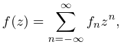
Let be analytic on the annulus , with Laurent expansion
| 2.10.25 | |||
| . | |||
What is the asymptotic behavior of as or ? More specially, what is the behavior of the higher coefficients in a Taylor-series expansion?
These problems can be brought within the scope of §2.4 by means of Cauchy’s integral formula
| 2.10.26 | |||
where is a simple closed contour in the annulus that encloses . For examples see Olver (1997b, Chapters 8, 9).
However, if is finite and has algebraic or logarithmic singularities on , then Darboux’s method is usually easier to apply. We need a “comparison function” with the properties:
-
(a)
is analytic on .
-
(b)
is continuous on .
-
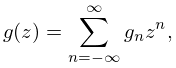
(c)
The coefficients in the Laurent expansion
2.10.27 , have known asymptotic behavior as .
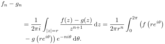
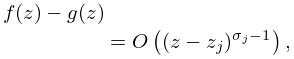
By allowing the contour in Cauchy’s formula to expand, we find that
| 2.10.28 | |||
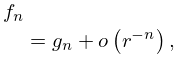
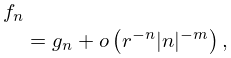
Hence by the Riemann–Lebesgue lemma (§1.8(i))
| 2.10.29 | |||
| . | |||
This result is refinable in two important ways. First, the conditions can be weakened. It is unnecessary for to be continuous on : it suffices that the integrals in (2.10.28) converge uniformly. For example, Condition (b) can be replaced by:
-
(b´)
On the circle , the function has a finite number of singularities, and at each singularity , say,
2.10.30 , where is a positive constant.
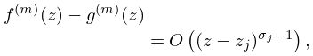
Secondly, when is times continuously differentiable on the result (2.10.29) can be strengthened. In these circumstances the integrals in (2.10.28) are integrable by parts times, yielding
| 2.10.31 | |||
| . | |||
Furthermore, (2.10.31) remains valid with the weaker condition
| 2.10.32 | |||
in the neighborhood of each singularity , again with .
Example
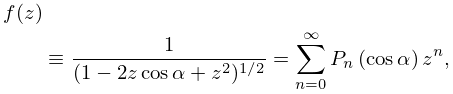
Let be a constant in and denote the Legendre polynomial of degree . From §14.7(iv)
| 2.10.33 | |||
| . | |||
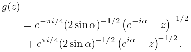
The singularities of on the unit circle are branch points at . To match the limiting behavior of at these points we set
| 2.10.34 | |||
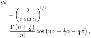
Here the branch of is continuous in the -plane cut along the outward-drawn ray through and equals at . Similarly for . In Condition (c) we have
| 2.10.35 | |||
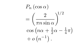
and in the supplementary conditions we may set . Then from (2.10.31) and (5.11.7)
| 2.10.36 | |||
For higher terms see §18.15(iii).
For uniform expansions when two singularities coalesce on the circle of convergence see Wong and Zhao (2005).
