Gauss 2F1(-1) sum
(0.011 seconds)
1—10 of 818 matching pages
1: 32.10 Special Function Solutions
…
►For example, if , with , then the Riccati equation is
…
►with , and , , independently.
…
►with and .
…
►where , , and , with , , independently.
…
►where , , , , and , with , , independently.
…
2: 16.10 Expansions in Series of Functions
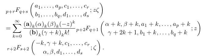
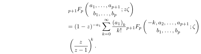
§16.10 Expansions in Series of Functions
… ►
16.10.1
…
►
16.10.2
►When the series on the right-hand side converges in the half-plane .
►Expansions of the form are discussed in Miller (1997), and further series of generalized hypergeometric functions are given in Luke (1969b, Chapter 9), Luke (1975, §§5.10.2 and 5.11), and Prudnikov et al. (1990, §§5.3, 6.8–6.9).
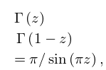
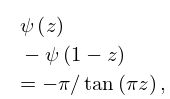
3: 5.5 Functional Relations
4: 15.4 Special Cases
…
►Exceptions are (15.4.8) and (15.4.10), that hold for , and (15.4.12), (15.4.14), and (15.4.16), that hold for .
…
►
§15.4(ii) Argument Unity
… ►Dougall’s Bilateral Sum
… ►§15.4(iii) Other Arguments
… ►where the limit interpretation (15.2.6), rather than (15.2.5), has to be taken when in (15.4.33) , and in (15.4.34) . …5: 15.5 Derivatives and Contiguous Functions
…
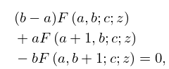
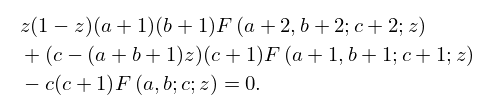
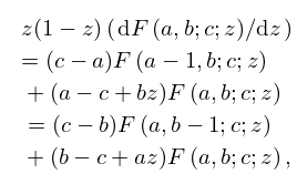
►The six functions , , are said to be contiguous to .
…
►
15.5.12
…
►By repeated applications of (15.5.11)–(15.5.18) any function , in which are integers, can be expressed as a linear combination of and any one of its contiguous functions, with coefficients that are rational functions of , and .
…
►
15.5.19
…
►
15.5.20
…
6: 18.33 Polynomials Orthogonal on the Unit Circle
…
►Instead of (18.33.9) one might take monic OP’s with weight function , and then express in terms of or .
…See Zhedanov (1998, §2).
…
►For the hypergeometric function see §§15.1 and 15.2(i).
…
►For the notation, including the basic hypergeometric function , see §§17.2 and 17.4(i).
…
►See Simon (2005a, p. 2, item (2)).
…
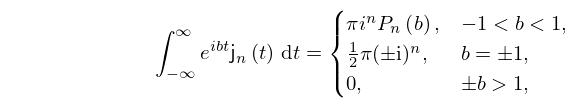
7: 10.59 Integrals
…
►
10.59.1
…
8: 19.21 Connection Formulas
…
►
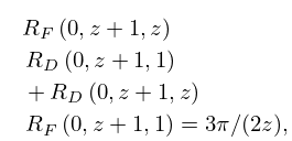
19.21.1
.
…
►The complete cases of and have connection formulas resulting from those for the Gauss hypergeometric function (Erdélyi et al. (1953a, §2.9)).
…
►
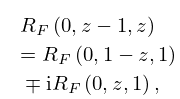
19.21.4
►
19.21.5
…
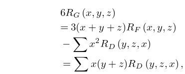
►
19.21.11
…
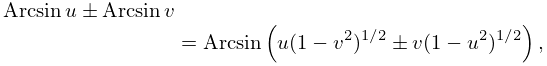
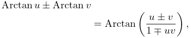
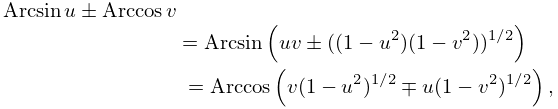
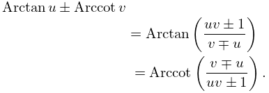
9: 4.24 Inverse Trigonometric Functions: Further Properties
10: 15.12 Asymptotic Approximations
…
►
(a)
…
►
(d)
►Then for fixed ,
…
►For the more general case in which and see Wagner (1990).
…
►By combination of the foregoing results of this subsection with the linear transformations of §15.8(i) and the connection formulas of §15.10(ii), similar asymptotic approximations for can be obtained with or , .
…
and/or .
and , where
15.12.1
with restricted so that .
