4 Elementary Functions Computation 4.44 Other Applications 4.46 Tables

§4.45 Methods of Computation

Permalink:: http://dlmf.nist.gov/4.45

§4.45(i) Real Variables
§4.45(ii) Complex Variables
§4.45(iii) Lambert $\mathop{W\/}\nolimits$ -Function

§4.45(i) Real Variables

Permalink:: http://dlmf.nist.gov/4.45.i

¶ Logarithms

Keywords:: logarithm function

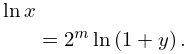
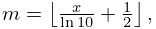
The function $\mathop{\ln\/}\nolimits x$ can always be computed from its ascending power series after preliminary scaling. Suppose first $1/10\leq x\leq 10$ . Then we take square roots repeatedly until is sufficiently small, where

4.45.1 $y=x^{{2^{{-m}}}}-1.$

Symbols:: : integer, : real variable and : real variable
Permalink:: http://dlmf.nist.gov/4.45.E1
Encodings:: TeX, pMML, png

After computing $\mathop{\ln\/}\nolimits\!\left(1+y\right)$ from (4.6.1)

4.45.2 $\mathop{\ln\/}\nolimits x=2^{m}\mathop{\ln\/}\nolimits\!\left(1+y\right).$

Symbols:: $\mathop{\ln\/}\nolimits z$ : principal branch of logarithm function, : integer, : real variable and : real variable
Permalink:: http://dlmf.nist.gov/4.45.E2
Encodings:: TeX, pMML, png

For other values of set $x=10^{m}\xi$ , where $1/10\leq\xi\leq 10$ and $m\in\Integer$ . Then

4.45.3 $\mathop{\ln\/}\nolimits x=\mathop{\ln\/}\nolimits\xi+m\mathop{\ln\/}\nolimits 10.$

Symbols:: $\mathop{\ln\/}\nolimits z$ : principal branch of logarithm function, : integer and : real variable
Permalink:: http://dlmf.nist.gov/4.45.E3
Encodings:: TeX, pMML, png

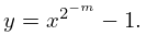
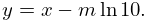
¶ Exponentials

Keywords:: exponential function

Let have any real value. First, rescale via

4.45.4

$m=\left\lfloor\frac{x}{\mathop{\ln\/}\nolimits 10}+\frac{1}{2}\right\rfloor,$

$y=x-m\mathop{\ln\/}\nolimits 10.$

Symbols:: $\left\lfloor x\right\rfloor$ : floor of , $\mathop{\ln\/}\nolimits z$ : principal branch of logarithm function, : integer, : real variable and : real variable
Permalink:: http://dlmf.nist.gov/4.45.E4
Encodings:: TeX, TeX, pMML, pMML, png, png

Then

4.45.5 $e^{x}=10^{m}e^{y},$

Symbols:: : base of exponential function, : integer, : real variable and : real variable
Permalink:: http://dlmf.nist.gov/4.45.E5
Encodings:: TeX, pMML, png

and since $|y|\leq\frac{1}{2}\mathop{\ln\/}\nolimits 10=1.15\dots$ , $e^{y}$ can be computed straightforwardly from (4.2.19).

¶ Trigonometric Functions

Keywords:: trigonometric functions

Let have any real value. We first compute $\xi=x/\pi$ , followed by

4.45.6

$m=\left\lfloor\xi+\tfrac{1}{2}\right\rfloor,$

$\theta=\pi(\xi-m).$

Symbols:: $\left\lfloor x\right\rfloor$ : floor of and : integer
Permalink:: http://dlmf.nist.gov/4.45.E6
Encodings:: TeX, TeX, pMML, pMML, png, png

Then

4.45.7

$\mathop{\sin\/}\nolimits x=(-1)^{m}\mathop{\sin\/}\nolimits\theta,$

$\mathop{\cos\/}\nolimits x=(-1)^{m}\mathop{\cos\/}\nolimits\theta,$

Symbols:: $\mathop{\cos\/}\nolimits z$ : cosine function, $\mathop{\sin\/}\nolimits z$ : sine function, : integer and : real variable
Permalink:: http://dlmf.nist.gov/4.45.E7
Encodings:: TeX, TeX, pMML, pMML, png, png

and since $|\theta|\leq\frac{1}{2}\pi=1.57\dots$ , $\mathop{\sin\/}\nolimits\theta$ and $\mathop{\cos\/}\nolimits\theta$ can be computed straightforwardly from (4.19.1) and (4.19.2).

The other trigonometric functions can be found from the definitions (4.14.4)–(4.14.7).

¶ Inverse Trigonometric Functions

Keywords:: inverse trigonometric functions

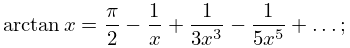
The function $\mathop{\mathrm{arctan}\/}\nolimits x$ can always be computed from its ascending power series after preliminary transformations to reduce the size of . From (4.24.15) with $u=v=((1+x^{2})^{{1/2}}-1)/x$ , we have

4.45.8 $2\mathop{\mathrm{arctan}\/}\nolimits\frac{(1+x^{2})^{{1/2}}-1}{x}=\mathop{% \mathrm{arctan}\/}\nolimits x,$ $0<x<\infty$ .

Symbols:: $\mathop{\mathrm{arctan}\/}\nolimits z$ : arctangent function and : real variable
Permalink:: http://dlmf.nist.gov/4.45.E8
Encodings:: TeX, pMML, png

Beginning with $x_{0}=x$ , generate the sequence

4.45.9 $x_{n}=\frac{(1+x^{2}_{{n-1}})^{{1/2}}-1}{x_{{n-1}}},$ $n=1,2,3,\dots$ ,

Symbols:: : integer and : real variable
Permalink:: http://dlmf.nist.gov/4.45.E9
Encodings:: TeX, pMML, png

until $x_{n}$ is sufficiently small. We then compute $\mathop{\mathrm{arctan}\/}\nolimits x_{n}$ from (4.24.3), followed by

4.45.10 $\mathop{\mathrm{arctan}\/}\nolimits x=2^{n}\mathop{\mathrm{arctan}\/}\nolimits x% _{n}.$

Symbols:: $\mathop{\mathrm{arctan}\/}\nolimits z$ : arctangent function, : integer and : real variable
Referenced by:: ¶ ‣ §4.45(i)
Permalink:: http://dlmf.nist.gov/4.45.E10
Encodings:: TeX, pMML, png

Another method, when is large, is to sum

4.45.11 $\mathop{\mathrm{arctan}\/}\nolimits x=\frac{\pi}{2}-\frac{1}{x}+\frac{1}{3x^{3% }}-\frac{1}{5x^{5}}+\dots;$

Symbols:: $\mathop{\mathrm{arctan}\/}\nolimits z$ : arctangent function and : real variable
Referenced by:: ¶ ‣ §4.45(i)
Permalink:: http://dlmf.nist.gov/4.45.E11
Encodings:: TeX, pMML, png

compare (4.24.4).

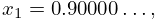
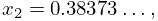
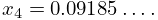
As an example, take . Then

4.45.12

$x_{1}=0.90000\dots,$

$x_{2}=0.38373\dots,$

$x_{3}=0.18528\dots,$

$x_{4}=0.09185\dots.$

Symbols:: : real variable
Permalink:: http://dlmf.nist.gov/4.45.E12
Encodings:: TeX, TeX, TeX, TeX, pMML, pMML, pMML, pMML, png, png, png, png

From (4.24.3) $\mathop{\mathrm{arctan}\/}\nolimits x_{4}=0.09160\dots$ . From (4.45.10)

4.45.13 $\mathop{\mathrm{arctan}\/}\nolimits x=16\mathop{\mathrm{arctan}\/}\nolimits x_% {4}=1.46563\dots.$

Symbols:: $\mathop{\mathrm{arctan}\/}\nolimits z$ : arctangent function and : real variable
Permalink:: http://dlmf.nist.gov/4.45.E13
Encodings:: TeX, pMML, png

As a check, from (4.45.11)

4.45.14 $\mathop{\mathrm{arctan}\/}\nolimits x=1.57079\ldots-0.10555\ldots+0.00039% \ldots-\cdots=1.46563\dots.$

Symbols:: $\mathop{\mathrm{arctan}\/}\nolimits z$ : arctangent function and : real variable
Permalink:: http://dlmf.nist.gov/4.45.E14
Encodings:: TeX, pMML, png

For the remaining inverse trigonometric functions, we may use the identities provided by the fourth row of Table 4.16.3. For example, $\mathop{\mathrm{arcsin}\/}\nolimits x=\mathop{\mathrm{arctan}\/}\nolimits\!% \left(x(1-x^{2})^{{-1/2}}\right)$ .

¶ Hyperbolic and Inverse Hyperbolic Functions

Keywords:: hyperbolic functions, inverse hyperbolic functions

The hyperbolic functions can be computed directly from the definitions (4.28.1)–(4.28.7). The inverses $\mathop{\mathrm{arcsinh}\/}\nolimits$ , $\mathop{\mathrm{arccosh}\/}\nolimits$ , and $\mathop{\mathrm{arctanh}\/}\nolimits$ can be computed from the logarithmic forms given in §4.37(iv), with real arguments. For $\mathop{\mathrm{arccsch}\/}\nolimits$ , $\mathop{\mathrm{arcsech}\/}\nolimits$ , and $\mathop{\mathrm{arccoth}\/}\nolimits$ we have (4.37.7)–(4.37.9).

¶ Other Methods

See Luther (1995), Ziv (1991), Cody and Waite (1980), Rosenberg and McNamee (1976), Carlson (1972a). For interval-arithmetic algorithms, see Markov (1981). For Shift-and-Add and CORDIC algorithms, see Muller (1997), Merrheim (1994), Schelin (1983). For multiprecision methods, see Smith (1989), Brent (1976).

§4.45(ii) Complex Variables

Permalink:: http://dlmf.nist.gov/4.45.ii

For $\mathop{\ln\/}\nolimits z$ and $e^{z}$

4.45.15 $\mathop{\ln\/}\nolimits z=\mathop{\ln\/}\nolimits|z|+i\mathop{\mathrm{ph}\/}% \nolimits z,$ $-\pi\leq\mathop{\mathrm{ph}\/}\nolimits z\leq\pi$ ,

Symbols:: $\mathop{\ln\/}\nolimits z$ : principal branch of logarithm function, $\mathop{\mathrm{ph}\/}\nolimits$ : phase and : complex variable
Permalink:: http://dlmf.nist.gov/4.45.E15
Encodings:: TeX, pMML, png

4.45.16 $e^{z}=e^{{\realpart{z}}}(\mathop{\cos\/}\nolimits\!\left(\imagpart{z}\right)+i% \mathop{\sin\/}\nolimits\!\left(\imagpart{z}\right)).$

Symbols:: $\mathop{\cos\/}\nolimits z$ : cosine function, : base of exponential function, $\imagpart{}$ : imaginary part, $\realpart{}$ : real part, $\mathop{\sin\/}\nolimits z$ : sine function and : complex variable
Permalink:: http://dlmf.nist.gov/4.45.E16
Encodings:: TeX, pMML, png

See §1.9(i) for the precise relationship of $\mathop{\mathrm{ph}\/}\nolimits z$ to the arctangent function.

The trigonometric functions may be computed from the definitions (4.14.1)–(4.14.7), and their inverses from the logarithmic forms in §4.23(iv), followed by (4.23.7)–(4.23.9). Similarly for the hyperbolic and inverse hyperbolic functions; compare (4.28.1)–(4.28.7), §4.37(iv), and (4.37.7)–(4.37.9).

For other methods see Miel (1981).

§4.45(iii) Lambert $\mathop{W\/}\nolimits$ -Function

Keywords:: Lambert $\mathop{W\/}\nolimits$ -function
Permalink:: http://dlmf.nist.gov/4.45.iii

For $x\in[-1/e,\infty)$ the principal branch $\mathop{\mathrm{Wp}\/}\nolimits\!\left(x\right)$ can be computed by solving the defining equation $We^{W}=x$ numerically, for example, by Newton’s rule (§3.8(ii)). Initial approximations are obtainable, for example, from the power series (4.13.6) (with $t\geq 0$ ) when is close to , from the asymptotic expansion (4.13.10) when is large, and by numerical integration of the differential equation (4.13.4) (§3.7) for other values of .