§4.23 Inverse Trigonometric Functions
Contents
- §4.23(i) General Definitions
- §4.23(ii) Principal Values
- §4.23(iii) Reflection Formulas
- §4.23(iv) Logarithmic Forms
- §4.23(v) Fundamental Property
- §4.23(vi) Real and Imaginary Parts
- §4.23(vii) Special Values and Interrelations
- §4.23(viii) Gudermannian Function
§4.23(i) General Definitions
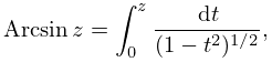
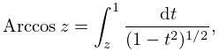
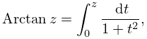
The general values of the inverse trigonometric functions are defined by
| 4.23.1 | ||||
| 4.23.2 | ||||
| 4.23.3 | ||||
| , | ||||
| 4.23.4 | ||||
| 4.23.5 | ||||
| 4.23.6 | ||||
In (4.23.1) and (4.23.2) the integration paths may not pass through either of the points . The function assumes its principal value when ; elsewhere on the integration paths the branch is determined by continuity. In (4.23.3) the integration path may not intersect . Each of the six functions is a multivalued function of . and have branch points at ; the other four functions have branch points at .
§4.23(ii) Principal Values
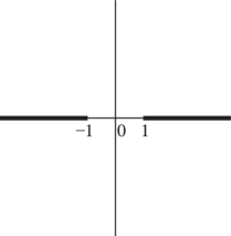
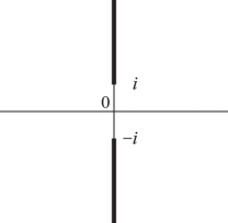
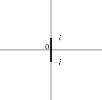
The principal values (or principal branches) of the inverse sine, cosine, and tangent are obtained by introducing cuts in the -plane as indicated in Figures 4.23.1(i) and 4.23.1(ii), and requiring the integration paths in (4.23.1)–(4.23.3) not to cross these cuts. Compare the principal value of the logarithm (§4.2(i)). The principal branches are denoted by , , , respectively. Each is two-valued on the corresponding cuts, and each is real on the part of the real axis that remains after deleting the intersections with the corresponding cuts.
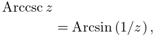
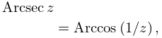
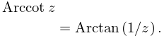
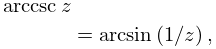
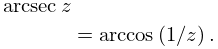
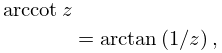
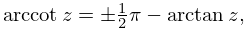
The principal values of the inverse cosecant, secant, and cotangent are given by
| 4.23.7 | ||||
| 4.23.8 | ||||
| 4.23.9 | ||||
| . | ||||
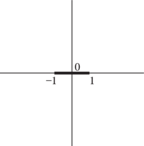
These functions are analytic in the cut plane depicted in Figures 4.23.1(iii) and 4.23.1(iv).
Except where indicated otherwise, it is assumed throughout the DLMF that the inverse trigonometric functions assume their principal values.
 |
 |
 |
 |
| (i) and | (ii) | (iii) and | (iv) |
Graphs of the principal values for real arguments are given in §4.15. This section also includes conformal mappings, and surface plots for complex arguments.
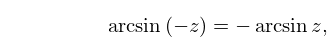
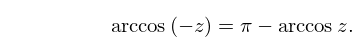
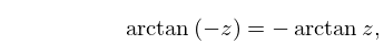
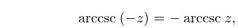
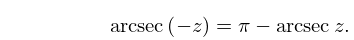
§4.23(iii) Reflection Formulas
| 4.23.10 | ||||
| 4.23.11 | ||||
| 4.23.12 | ||||
| . | ||||
| 4.23.13 | ||||
| 4.23.14 | ||||
| 4.23.15 | ||||
| . | ||||
| 4.23.16 | ||||
| 4.23.17 | ||||
| 4.23.18 | ||||
| . | ||||
§4.23(iv) Logarithmic Forms
Throughout this subsection all quantities assume their principal values.
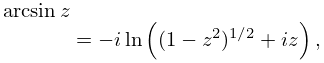
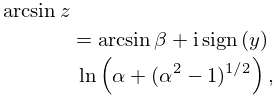
Inverse Sine
| 4.23.19 | |||
| ; | |||
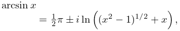
compare Figure 4.23.1(i). On the cuts
| 4.23.20 | ||||
| , | ||||
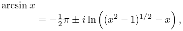
| 4.23.21 | ||||
| , | ||||
upper signs being taken on upper sides, and lower signs on lower sides.
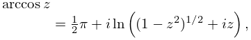
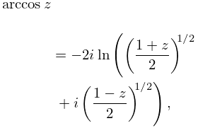
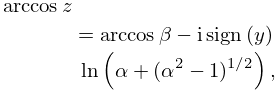
Inverse Cosine
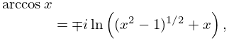
On the cuts
| 4.23.24 | ||||
| , | ||||
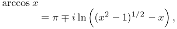
| 4.23.25 | ||||
| , | ||||
the upper/lower signs corresponding to the upper/lower sides.
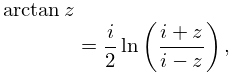
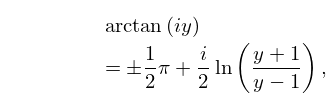
Inverse Tangent
| 4.23.26 | |||
| ; | |||
compare Figure 4.23.1(ii). On the cuts
| 4.23.27 | |||
| , | |||
the upper/lower sign corresponding to the right/left side.
Other Inverse Functions
§4.23(v) Fundamental Property
With , the general solutions of the equations
| 4.23.28 | ||||
| 4.23.29 | ||||
| 4.23.30 | ||||
are respectively
| 4.23.31 | ||||
| 4.23.32 | ||||
| 4.23.33 | ||||
| . | ||||
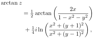
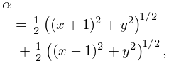
§4.23(vi) Real and Imaginary Parts
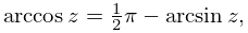
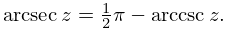
§4.23(vii) Special Values and Interrelations
| – | – | |||||
| – | – | |||||
| – | – |
For interrelations see Table 4.16.3. For example, from the heading and last entry in the penultimate column we have .
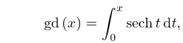
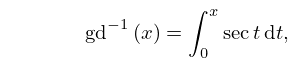
§4.23(viii) Gudermannian Function
The Gudermannian is defined by
| 4.23.39 | |||
| . | |||
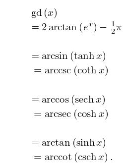
Equivalently,
| 4.23.40 | |||
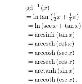
The inverse Gudermannian function is given by
| 4.23.41 | |||
| . | |||
Equivalently, and again when ,
| 4.23.42 | |||
