.威尼斯赌场『wn4.com』澳门威尼斯赌场.威尼斯线上赌场.真的威尼斯赌场.威尼斯娱乐.威尼斯真人.威尼斯棋牌-w6n2c9o.2022年11月30日1时19分46秒.6yuks2eos.com

♦ 21—30 of 147 matching pages ♦

(0.003 seconds)

21—30 of 147 matching pages

21: Bibliography G

… ►

W. Gautschi (1966) Algorithm 292: Regular Coulomb wave functions. Comm. ACM 9 (11), pp. 793–795.

ⓘ

External Links:: ISSN 0001-0782, Document
Referenced by:: §33.26(ii).
Encodings:: BibTeX

►

W. Gautschi (1969) Algorithm 363: Complex error function. Comm. ACM 12 (11), pp. 635.

ⓘ

Notes:: Includes Algol program, maximum accuracy 10S. For certification see same journal v. 15 (1972), pp. 465–466
External Links:: ISSN 0001-0782, Document
Referenced by:: §7.25(iii).
Encodings:: BibTeX

… ►

A. Gil, J. Segura, and N. M. Temme (2002c) Computing complex Airy functions by numerical quadrature. Numer. Algorithms 30 (1), pp. 11–23.

ⓘ

External Links:: ISSN 1017-1398, Document, MathReview (Richard B. Paris), ZentralBlatt
Referenced by:: §9.17(iii).
Encodings:: BibTeX

… ►

H. W. Gould (1960) Stirling number representation problems. Proc. Amer. Math. Soc. 11 (3), pp. 447–451.

ⓘ

External Links:: FullText, MathReview (L. Carlitz), ZentralBlatt
Referenced by:: §26.1, §26.1, Notations S, Notations S.
Encodings:: BibTeX

… ►

V. I. Gromak (1975) Theory of Painlevé’s equations. Differ. Uravn. 11 (11), pp. 373–376 (Russian).

ⓘ

Notes:: In Russian. English translation: Differential Equations 11(11), pp. 285–287
External Links:: MathReview (Z. Nehari), ZentralBlatt
Referenced by:: §32.7(iii), §32.7(vi).
Encodings:: BibTeX

…

P. Deift, T. Kriecherbauer, K. T.-R. McLaughlin, S. Venakides, and X. Zhou (1999b) Uniform asymptotics for polynomials orthogonal with respect to varying exponential weights and applications to universality questions in random matrix theory. Comm. Pure Appl. Math. 52 (11), pp. 1335–1425.

ⓘ

External Links:: ISSN 0010-3640, Document, MathReview (D. S. Lubinsky), ZentralBlatt
Referenced by:: §18.32.
Encodings:: BibTeX

… ►

S. C. Dhar (1940) Note on the addition theorem of parabolic cylinder functions. J. Indian Math. Soc. (N. S.) 4, pp. 29–30.

ⓘ

External Links:: MathReview (M. C. Gray), ZentralBlatt
Referenced by:: §12.13(ii).
Encodings:: BibTeX

… ►

E. Dorrer (1968) Algorithm 322. F-distribution. Comm. ACM 11 (2), pp. 116–117.

ⓘ

Notes:: Includes Algol program, maximum accuracy 10S. For certification see same journal 12(1969), p. 39
External Links:: ISSN 0001-0782, Document
Referenced by:: §8.28(iv).
Encodings:: BibTeX

… ►

B. A. Dubrovin (1981) Theta functions and non-linear equations. Uspekhi Mat. Nauk 36 (2(218)), pp. 11–80 (Russian).

ⓘ

Notes:: With an appendix by I. M. Krichever. In Russian. English translation: Russian Math. Surveys 36(1981), no. 2, pp. 11–92 (1982)
External Links:: ISSN 0042-1316, Document, MathReview (Alexander A. Pankov), ZentralBlatt
Referenced by:: §21.1, §21.6(ii), §21.7(i), Figure 21.9.2, Figure 21.9.2, §21.9, §21.9, Sidebar 21.SB2, Ch.21, Notations T.
Encodings:: BibTeX

… ►

J. Dutka (1981) The incomplete beta function—a historical profile. Arch. Hist. Exact Sci. 24 (1), pp. 11–29.

ⓘ

External Links:: ISSN 0003-9519, MathReview (Willard Parker), ZentralBlatt
Referenced by:: §8.17(i).
Encodings:: BibTeX

…

23: Bibliography C

… ►

L. Carlitz (1960) Note on Nörlund’s polynomial

B_{n}^{(z)}

. Proc. Amer. Math. Soc. 11 (3), pp. 452–455.

ⓘ

External Links:: FullText, MathReview (M. P. Drazin), ZentralBlatt
Referenced by:: §26.1, §26.1, Notations S, Notations S.
Encodings:: BibTeX

… ►

P. A. Clarkson (2003b) The fourth Painlevé equation and associated special polynomials. J. Math. Phys. 44 (11), pp. 5350–5374.

ⓘ

External Links:: ISSN 0022-2488, Document, MathReview, ZentralBlatt
Referenced by:: §32.8(iv).
Encodings:: BibTeX

… ►

J. A. Cochran (1963) Further formulas for calculating approximate values of the zeros of certain combinations of Bessel functions. IEEE Trans. Microwave Theory Tech. 11 (6), pp. 546–547.

ⓘ

External Links:: ISSN 0018-9480, FullText
Referenced by:: §10.21(x).
Encodings:: BibTeX

… ►

M. Colman, A. Cuyt, and J. Van Deun (2011) Validated computation of certain hypergeometric functions. ACM Trans. Math. Software 38 (2), pp. Art. 11, 20.

ⓘ

External Links:: ISSN 0098-3500, Document, FullText, MathReview Entry, ZentralBlatt
Referenced by:: §13.29(v), §15.19(v).
Encodings:: BibTeX

… ►

F. Cooper, A. Khare, and A. Saxena (2006) Exact elliptic compactons in generalized Korteweg-de Vries equations. Complexity 11 (6), pp. 30–34.

ⓘ

External Links:: ISSN 1076-2787, Document, MathReview
Referenced by:: §19.6(i).
Encodings:: BibTeX

…

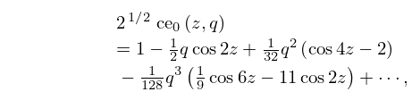
24: 28.6 Expansions for Small $q$

… ►

28.6.2

a_{1}\left(q\right)=1+q-\tfrac{1}{8}q^{2}-\tfrac{1}{64}q^{3}-\tfrac{1}{1536}q^% {4}+\tfrac{11}{36864}q^{5}+\tfrac{49}{5\;89824}q^{6}+\tfrac{55}{94\;37184}q^{7% }-\tfrac{83}{353\;89440}q^{8}+\cdots,

ⓘ

Symbols:: $a_{\NVar{n}}\left(\NVar{q}\right)$ : eigenvalues of Mathieu equation and $q=h^{2}$ : parameter
Permalink:: http://dlmf.nist.gov/28.6.E2
Encodings:: pMML, png, TeX
See also:: Annotations for §28.6(i), §28.6 and Ch.28

►

28.6.3

b_{1}\left(q\right)=1-q-\tfrac{1}{8}q^{2}+\tfrac{1}{64}q^{3}-\tfrac{1}{1536}q^% {4}-\tfrac{11}{36864}q^{5}+\tfrac{49}{5\;89824}q^{6}-\tfrac{55}{94\;37184}q^{7% }-\tfrac{83}{353\;89440}q^{8}+\cdots,

ⓘ

Symbols:: $b_{\NVar{n}}\left(\NVar{q}\right)$ : eigenvalues of Mathieu equation and $q=h^{2}$ : parameter
Permalink:: http://dlmf.nist.gov/28.6.E3
Encodings:: pMML, png, TeX
See also:: Annotations for §28.6(i), §28.6 and Ch.28

… ►

28.6.10

a_{5}\left(q\right)=25+\tfrac{1}{48}q^{2}+\tfrac{11}{7\;74144}q^{4}+\tfrac{1}{% 1\;47456}q^{5}+\tfrac{37}{8918\;13888}q^{6}+\cdots,

ⓘ

Symbols:: $a_{\NVar{n}}\left(\NVar{q}\right)$ : eigenvalues of Mathieu equation and $q=h^{2}$ : parameter
Permalink:: http://dlmf.nist.gov/28.6.E10
Encodings:: pMML, png, TeX
See also:: Annotations for §28.6(i), §28.6 and Ch.28

►

28.6.11

b_{5}\left(q\right)=25+\tfrac{1}{48}q^{2}+\tfrac{11}{7\;74144}q^{4}-\tfrac{1}{% 1\;47456}q^{5}+\tfrac{37}{8918\;13888}q^{6}+\cdots,

ⓘ

Symbols:: $b_{\NVar{n}}\left(\NVar{q}\right)$ : eigenvalues of Mathieu equation and $q=h^{2}$ : parameter
Permalink:: http://dlmf.nist.gov/28.6.E11
Encodings:: pMML, png, TeX
See also:: Annotations for §28.6(i), §28.6 and Ch.28

… ►

28.6.21

2^{\ifrac{1}{2}}\operatorname{ce}_{0}\left(z,q\right)=1-\tfrac{1}{2}q\cos 2z+% \tfrac{1}{32}q^{2}\left(\cos 4z-2\right)-\tfrac{1}{128}q^{3}\left(\tfrac{1}{9}% \cos 6z-11\cos 2z\right)+\cdots,

ⓘ

Symbols:: $\operatorname{ce}_{\NVar{n}}\left(\NVar{z},\NVar{q}\right)$ : Mathieu function, $\cos\NVar{z}$ : cosine function, $q=h^{2}$ : parameter and $z$ : complex variable
A&S Ref:: 20.2.27
Referenced by:: §28.6(ii)
Permalink:: http://dlmf.nist.gov/28.6.E21
Encodings:: pMML, png, TeX
See also:: Annotations for §28.6(ii), §28.6 and Ch.28

…

25: Bibliography O

… ►

K. Okamoto (1987c) Studies on the Painlevé equations. IV. Third Painlevé equation

P_{{\rm III}}

. Funkcial. Ekvac. 30 (2-3), pp. 305–332.

ⓘ

External Links:: ISSN 0532-8721, FullText, MathReview (Hélène Airault), ZentralBlatt
Referenced by:: §32.10(iii), §32.2(iii), §32.6(iv), §32.7(viii).
Encodings:: BibTeX

… ►

F. W. J. Olver (1950) A new method for the evaluation of zeros of Bessel functions and of other solutions of second-order differential equations. Proc. Cambridge Philos. Soc. 46 (4), pp. 570–580.

ⓘ

External Links:: Document, MathReview (J. Todd), ZentralBlatt
Referenced by:: §10.21(ii).
Encodings:: BibTeX

… ►

S. Olver (2011) Numerical solution of Riemann-Hilbert problems: Painlevé II. Found. Comput. Math. 11 (2), pp. 153–179.

ⓘ

External Links:: ISSN 1615-3375, Document, FullText, MathReview Entry, ZentralBlatt
Referenced by:: §32.17, §32.17.
Encodings:: BibTeX

… ►

H. Oser (1960) Algorithm 22: Riccati-Bessel functions of first and second kind. Comm. ACM 3 (11), pp. 600–601.

ⓘ

Notes:: Includes Algol code, minimum accuracy 9S. For certification see same journal 13(1970), p. 448.
External Links:: ISSN 0001-0782, Document
Referenced by:: §10.77(ii).
Encodings:: BibTeX

…

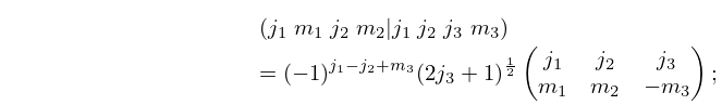
26: 34.1 Special Notation

… ►

\begin{Bmatrix}j_{11}&j_{12}&j_{13}\\ j_{21}&j_{22}&j_{23}\\ j_{31}&j_{32}&j_{33}\end{Bmatrix}.

… ►

34.1.1

\left(j_{1}\;m_{1}\;j_{2}\;m_{2}|j_{1}\;j_{2}\;j_{3}\,\,m_{3}\right)=(-1)^{j_{% 1}-j_{2}+m_{3}}(2j_{3}+1)^{\frac{1}{2}}\begin{pmatrix}j_{1}&j_{2}&j_{3}\\ m_{1}&m_{2}&-m_{3}\end{pmatrix};

ⓘ

Symbols:: $\begin{pmatrix}\NVar{j_{1}}&\NVar{j_{2}}&\NVar{j_{3}}\\ \NVar{m_{1}}&\NVar{m_{2}}&\NVar{m_{3}}\end{pmatrix}$ : $\mathit{3j}$ symbol and $j,j_{r}$ : non-negative integers or non-negative integers plus one half.
Sources:: Edmonds (1974, p. 46, Eq. (3.7.3)); Rotenberg et al. (1959, p. 1, Eq. (1.1a))
Permalink:: http://dlmf.nist.gov/34.1.E1
Encodings:: pMML, png, TeX
Clarification (effective with 1.0.15):: A wording change reflects that the Clebsch–Gordan coefficients are an alternative formulation of angular momentum problems, rather than alternative notation for the $\mathit{3j}$ . The sign of $m_{3}$ was changed for clarity.
See also:: Annotations for §34.1 and Ch.34

►see Edmonds (1974, p. 46, Eq. (3.7.3)) and Rotenberg et al. (1959, p. 1, Eq. (1.1a)). …

27: Bibliography F

… ►

B. R. Fabijonas (2004) Algorithm 838: Airy functions. ACM Trans. Math. Software 30 (4), pp. 491–501.

ⓘ

Notes:: Single- and double-precision Fortran, maximum accuracy 32S.
External Links:: ISSN 0098-3500, Document, Code, MathReview Entry, ZentralBlatt
Referenced by:: 3rd item, 2nd item, 1st item.
Encodings:: BibTeX

… ►

N. Fleury and A. Turbiner (1994) Polynomial relations in the Heisenberg algebra. J. Math. Phys. 35 (11), pp. 6144–6149.

ⓘ

External Links:: ISSN 0022-2488, Document, MathReview (Shao-Ming Fei), ZentralBlatt
Referenced by:: §13.3(ii), §15.5(i), §16.3(i).
Encodings:: BibTeX

… ►

A. S. Fokas and M. J. Ablowitz (1982) On a unified approach to transformations and elementary solutions of Painlevé equations. J. Math. Phys. 23 (11), pp. 2033–2042.

ⓘ

External Links:: ISSN 0022-2488, Document, MathReview (Hélène Airault), ZentralBlatt
Referenced by:: §32.13(i), §32.7(i), §32.7(iii).
Encodings:: BibTeX

… ►

A. S. Fokas and Y. C. Yortsos (1981) The transformation properties of the sixth Painlevé equation and one-parameter families of solutions. Lett. Nuovo Cimento (2) 30 (17), pp. 539–544.

ⓘ

External Links:: ISSN 0024-1318, MathReview (D. A. Lutz)
Referenced by:: §32.10(vi).
Encodings:: BibTeX

… ►

L. W. Fullerton (1972) Algorithm 435: Modified incomplete gamma function. Comm. ACM 15 (11), pp. 993–995.

ⓘ

Notes:: Includes Fortran code. For a Remark see ACM Trans. Math. Software 4 (1978), no. 3, pp. 296–304.
External Links:: ISSN 0001-0782, Document, Remark
Referenced by:: §8.28(ii).
Encodings:: BibTeX

…

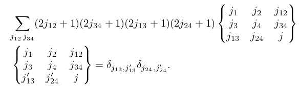
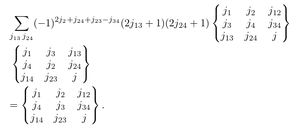
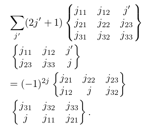
28: 34.7 Basic Properties: $\mathit{9j}$ Symbol

… ►

34.7.1

\begin{Bmatrix}j_{11}&j_{12}&j_{13}\\ j_{21}&j_{22}&j_{13}\\ j_{31}&j_{31}&0\end{Bmatrix}=\frac{(-1)^{j_{12}+j_{21}+j_{13}+j_{31}}}{((2j_{1% 3}+1)(2j_{31}+1))^{\frac{1}{2}}}\begin{Bmatrix}j_{11}&j_{12}&j_{13}\\ j_{22}&j_{21}&j_{31}\end{Bmatrix}.

ⓘ

Symbols:: $\begin{Bmatrix}\NVar{j_{11}}&\NVar{j_{12}}&\NVar{j_{13}}\\ \NVar{j_{21}}&\NVar{j_{22}}&\NVar{j_{23}}\\ \NVar{j_{31}}&\NVar{j_{32}}&\NVar{j_{33}}\end{Bmatrix}$ : $\mathit{9j}$ symbol, $\begin{Bmatrix}\NVar{j_{1}}&\NVar{j_{2}}&\NVar{j_{3}}\\ \NVar{l_{1}}&\NVar{l_{2}}&\NVar{l_{3}}\end{Bmatrix}$ : $\mathit{6j}$ symbol and $j,j_{r}$ : non-negative integers or non-negative integers plus one half.
Permalink:: http://dlmf.nist.gov/34.7.E1
Encodings:: pMML, png, TeX
See also:: Annotations for §34.7(i), §34.7 and Ch.34

… ►

34.7.2

\sum_{j_{12}\,j_{34}}(2j_{12}+1)(2j_{34}+1)(2j_{13}+1)(2j_{24}+1)\begin{% Bmatrix}j_{1}&j_{2}&j_{12}\\ j_{3}&j_{4}&j_{34}\\ j_{13}&j_{24}&j\end{Bmatrix}\begin{Bmatrix}j_{1}&j_{2}&j_{12}\\ j_{3}&j_{4}&j_{34}\\ j^{\prime}_{13}&j^{\prime}_{24}&j\end{Bmatrix}=\delta_{j_{13},j^{\prime}_{13}}% \delta_{j_{24},j^{\prime}_{24}}.

ⓘ

Symbols:: $\delta_{\NVar{j},\NVar{k}}$ : Kronecker delta, $\begin{Bmatrix}\NVar{j_{11}}&\NVar{j_{12}}&\NVar{j_{13}}\\ \NVar{j_{21}}&\NVar{j_{22}}&\NVar{j_{23}}\\ \NVar{j_{31}}&\NVar{j_{32}}&\NVar{j_{33}}\end{Bmatrix}$ : $\mathit{9j}$ symbol and $j,j_{r}$ : non-negative integers or non-negative integers plus one half.
Permalink:: http://dlmf.nist.gov/34.7.E2
Encodings:: pMML, png, TeX
See also:: Annotations for §34.7(iv), §34.7 and Ch.34

… ►

34.7.3

\sum_{j_{13}\,j_{24}}(-1)^{2j_{2}+j_{24}+j_{23}-j_{34}}(2j_{13}+1)(2j_{24}+1)% \begin{Bmatrix}j_{1}&j_{2}&j_{12}\\ j_{3}&j_{4}&j_{34}\\ j_{13}&j_{24}&j\end{Bmatrix}\begin{Bmatrix}j_{1}&j_{3}&j_{13}\\ j_{4}&j_{2}&j_{24}\\ j_{14}&j_{23}&j\end{Bmatrix}=\begin{Bmatrix}j_{1}&j_{2}&j_{12}\\ j_{4}&j_{3}&j_{34}\\ j_{14}&j_{23}&j\end{Bmatrix}.

ⓘ

Symbols:: $\begin{Bmatrix}\NVar{j_{11}}&\NVar{j_{12}}&\NVar{j_{13}}\\ \NVar{j_{21}}&\NVar{j_{22}}&\NVar{j_{23}}\\ \NVar{j_{31}}&\NVar{j_{32}}&\NVar{j_{33}}\end{Bmatrix}$ : $\mathit{9j}$ symbol and $j,j_{r}$ : non-negative integers or non-negative integers plus one half.
Referenced by:: §34.9
Permalink:: http://dlmf.nist.gov/34.7.E3
Encodings:: pMML, png, TeX
See also:: Annotations for §34.7(vi), §34.7 and Ch.34

… ►

34.7.4

\begin{pmatrix}j_{13}&j_{23}&j_{33}\\ m_{13}&m_{23}&m_{33}\end{pmatrix}\begin{Bmatrix}j_{11}&j_{12}&j_{13}\\ j_{21}&j_{22}&j_{23}\\ j_{31}&j_{32}&j_{33}\end{Bmatrix}=\sum_{m_{r1},m_{r2},r=1,2,3}\begin{pmatrix}j% _{11}&j_{12}&j_{13}\\ m_{11}&m_{12}&m_{13}\end{pmatrix}\begin{pmatrix}j_{21}&j_{22}&j_{23}\\ m_{21}&m_{22}&m_{23}\end{pmatrix}\*\begin{pmatrix}j_{31}&j_{32}&j_{33}\\ m_{31}&m_{32}&m_{33}\end{pmatrix}\begin{pmatrix}j_{11}&j_{21}&j_{31}\\ m_{11}&m_{21}&m_{31}\end{pmatrix}\begin{pmatrix}j_{12}&j_{22}&j_{32}\\ m_{12}&m_{22}&m_{32}\end{pmatrix}.

ⓘ

Symbols:: $\begin{Bmatrix}\NVar{j_{11}}&\NVar{j_{12}}&\NVar{j_{13}}\\ \NVar{j_{21}}&\NVar{j_{22}}&\NVar{j_{23}}\\ \NVar{j_{31}}&\NVar{j_{32}}&\NVar{j_{33}}\end{Bmatrix}$ : $\mathit{9j}$ symbol, $\begin{pmatrix}\NVar{j_{1}}&\NVar{j_{2}}&\NVar{j_{3}}\\ \NVar{m_{1}}&\NVar{m_{2}}&\NVar{m_{3}}\end{pmatrix}$ : $\mathit{3j}$ symbol, $j,j_{r}$ : non-negative integers or non-negative integers plus one half. and $r$ : nonnegative integer
Referenced by:: Erratum (V1.0.10) for Equation (34.7.4)
Permalink:: http://dlmf.nist.gov/34.7.E4
Encodings:: pMML, png, TeX
Errata (effective with 1.0.10):: Originally the third $\mathit{3j}$ symbol in the summation was written incorrectly as $\begin{pmatrix}j_{31}&j_{32}&j_{33}\\ m_{13}&m_{23}&m_{33}\end{pmatrix}.$
Reported 2015-01-19 by Yan-Rui Liu
See also:: Annotations for §34.7(vi), §34.7 and Ch.34

►

34.7.5

\sum_{j^{\prime}}(2j^{\prime}+1)\begin{Bmatrix}j_{11}&j_{12}&j^{\prime}\\ j_{21}&j_{22}&j_{23}\\ j_{31}&j_{32}&j_{33}\end{Bmatrix}\begin{Bmatrix}j_{11}&j_{12}&j^{\prime}\\ j_{23}&j_{33}&j\end{Bmatrix}={(-1)^{2j}}\begin{Bmatrix}j_{21}&j_{22}&j_{23}\\ j_{12}&j&j_{32}\end{Bmatrix}\begin{Bmatrix}j_{31}&j_{32}&j_{33}\\ j&j_{11}&j_{21}\end{Bmatrix}.

ⓘ

Symbols:: $\begin{Bmatrix}\NVar{j_{11}}&\NVar{j_{12}}&\NVar{j_{13}}\\ \NVar{j_{21}}&\NVar{j_{22}}&\NVar{j_{23}}\\ \NVar{j_{31}}&\NVar{j_{32}}&\NVar{j_{33}}\end{Bmatrix}$ : $\mathit{9j}$ symbol, $\begin{Bmatrix}\NVar{j_{1}}&\NVar{j_{2}}&\NVar{j_{3}}\\ \NVar{l_{1}}&\NVar{l_{2}}&\NVar{l_{3}}\end{Bmatrix}$ : $\mathit{6j}$ symbol and $j,j_{r}$ : non-negative integers or non-negative integers plus one half.
Permalink:: http://dlmf.nist.gov/34.7.E5
Encodings:: pMML, png, TeX
See also:: Annotations for §34.7(vi), §34.7 and Ch.34

29: Bibliography L

… ►

D. Le (1985) An efficient derivative-free method for solving nonlinear equations. ACM Trans. Math. Software 11 (3), pp. 250–262.

ⓘ

Notes:: Corrigendum, ibid. 15(3) (1989), 287
External Links:: ISSN 0098-3500, Document, MathReview (T. Feagin), ZentralBlatt
Referenced by:: §3.8(iii).
Encodings:: BibTeX

… ►

A. Leitner and J. Meixner (1960) Eine Verallgemeinerung der Sphäroidfunktionen. Arch. Math. 11, pp. 29–39.

ⓘ

External Links:: ISSN 0003-9268, Document, MathReview (M. J. O. Strutt), ZentralBlatt
Referenced by:: §30.12.
Encodings:: BibTeX

… ►

H. Lotsch and M. Gray (1964) Algorithm 244: Fresnel integrals. Comm. ACM 7 (11), pp. 660–661.

ⓘ

Notes:: Includes Algol program, maximum accuracy 12D.
External Links:: ISSN 0001-0782, Document
Referenced by:: §7.25(iv).
Encodings:: BibTeX

… ►

N. A. Lukaševič (1967b) On the theory of Painlevé’s third equation. Differ. Uravn. 3 (11), pp. 1913–1923 (Russian).

ⓘ

Notes:: In Russian. English translation: Differential Equations 3(11), pp. 994–999
External Links:: MathReview (Z. Nehari), ZentralBlatt
Referenced by:: §32.10(iii), §32.8(iii), §32.9(i), §32.9(ii).
Encodings:: BibTeX

… ►

Y. L. Luke (1977a) Algorithms for rational approximations for a confluent hypergeometric function. Utilitas Math. 11, pp. 123–151.

ⓘ

External Links:: MathReview (F. Gotze), ZentralBlatt
Referenced by:: §13.31(iii).
Encodings:: BibTeX

…

30: 9.18 Tables

… ►

•

Miller (1946) tabulates $\operatorname{Ai}\left(x\right)$ , $\operatorname{Ai}'\left(x\right)$ for $x=-20(.01)2;$ $\operatorname{log}_{10}\operatorname{Ai}\left(x\right)$ , $\operatorname{Ai}'\left(x\right)/\operatorname{Ai}\left(x\right)$ for $x=0(.1)25(1)75$ ; $\operatorname{Bi}\left(x\right)$ , $\operatorname{Bi}'\left(x\right)$ for $x=-10(.1)2.5$ ; $\operatorname{log}_{10}\operatorname{Bi}\left(x\right)$ , $\operatorname{Bi}'\left(x\right)/\operatorname{Bi}\left(x\right)$ for $x=0(.1)10$ ; $M\left(x\right)$ , $N\left(x\right)$ , $\theta\left(x\right)$ , $\phi\left(x\right)$ (respectively $F(x)$ , $G(x)$ , $\chi(x)$ , $\psi(x)$ ) for $x=-80(1)-30(.1)0$ . Precision is generally 8D; slightly less for some of the auxiliary functions. Extracts from these tables are included in Abramowitz and Stegun (1964, Chapter 10), together with some auxiliary functions for large arguments.

… ►

•

National Bureau of Standards (1958) tabulates $A_{0}(x)\equiv\pi\operatorname{Hi}\left(-x\right)$ and $-A_{0}^{\prime}(x)\equiv\pi\operatorname{Hi}'\left(-x\right)$ for $x=0(.01)1(.02)5(.05)11$ and $1/x=0.01(.01)0.1$ ; $\int_{0}^{x}A_{0}(t)\,\mathrm{d}t$ for $x=0.5,1(1)11$ . Precision is 8D.

… ►

•

Gil et al. (2003c) tabulates the only positive zero of $\operatorname{Gi}'\left(z\right)$ , the first 10 negative real zeros of $\operatorname{Gi}\left(z\right)$ and $\operatorname{Gi}'\left(z\right)$ , and the first 10 complex zeros of $\operatorname{Gi}\left(z\right)$ , $\operatorname{Gi}'\left(z\right)$ , $\operatorname{Hi}\left(z\right)$ , and $\operatorname{Hi}'\left(z\right)$ . Precision is 11 or 12S.

…