Gauss formula
(0.002 seconds)
21—30 of 50 matching pages
21: 35.9 Applications
…
►In multivariate statistical analysis based on the multivariate normal distribution, the probability density functions of many random matrices are expressible in terms of generalized hypergeometric functions of matrix argument , with and .
…
►For other statistical applications of functions of matrix argument see Perlman and Olkin (1980), Groeneboom and Truax (2000), Bhaumik and Sarkar (2002), Richards (2004) (monotonicity of power functions of multivariate statistical test criteria), Bingham et al. (1992) (Procrustes analysis), and Phillips (1986) (exact distributions of statistical test criteria).
These references all use results related to the integral formulas (35.4.7) and (35.5.8).
…
22: 15.5 Derivatives and Contiguous Functions
…
►
§15.5(i) Differentiation Formulas
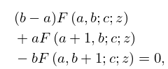
… ►The six functions , , are said to be contiguous to . … ►
15.5.12
…
►By repeated applications of (15.5.11)–(15.5.18) any function , in which are integers, can be expressed as a linear combination of and any one of its contiguous functions, with coefficients that are rational functions of , and .
…
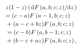
►
15.5.20
…
23: 15.6 Integral Representations
…
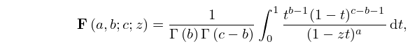
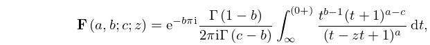
►The function (not ) has the following integral representations:
►
15.6.1
; .
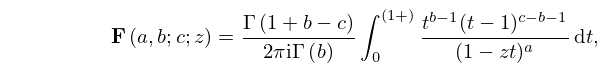
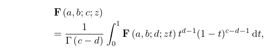
►
15.6.2
; , .
…
►
15.6.3
; , .
…
►
15.6.8
; .
…
24: 18.35 Pollaczek Polynomials
…
►
18.35.4
…
25: Bibliography V
…
►
Some Wonderful Formulas
an Introduction to Polylogarithms.
In Proceedings of the Queen’s Number Theory Conference, 1979
(Kingston, Ont., 1979), R. Ribenboim (Ed.),
Queen’s Papers in Pure and Appl. Math., Vol. 54, Kingston, Ont., pp. 269–286.
…
►
Certain summation formulae for -series.
J. Indian Math. Soc. (N.S.) 47 (1-4), pp. 71–85 (1986).
…
►
Transformations of some Gauss hypergeometric functions.
J. Comput. Appl. Math. 178 (1-2), pp. 473–487.
…
26: 15.10 Hypergeometric Differential Equation
…
►
…
►
…
►(b) If equals , and , then fundamental solutions in the neighborhood of are given by and
…
►
§15.10(ii) Kummer’s 24 Solutions and Connection Formulas
… ►The connection formulas for the principal branches of Kummer’s solutions are: …27: 15.8 Transformations of Variable
…
►The transformation formulas between two hypergeometric functions in Group 2, or two hypergeometric functions in Group 3, are the linear transformations (15.8.1).
…
►
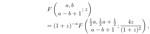
15.8.13
,
►
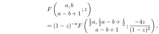
15.8.14
.
…
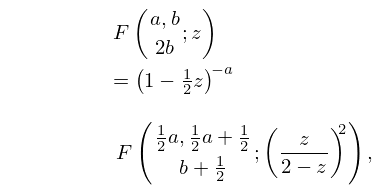
►
15.8.15
,
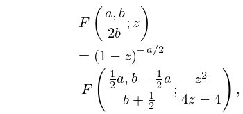
►
15.8.16
.
…
28: 17.7 Special Cases of Higher Functions
…
►
-Analog of Bailey’s Sum
… ►-Analog of Gauss’s Sum
… ►-Analog of Dixon’s Sum
… ►Gasper–Rahman -Analog of Watson’s Sum
… ►Second -Analog of Bailey’s Sum
…29: Bibliography M
…
►
A determinant formula for a class of rational solutions of Painlevé V equation.
Nagoya Math. J. 168, pp. 1–25.
►
On a class of algebraic solutions to the Painlevé VI equation, its determinant formula and coalescence cascade.
Funkcial. Ekvac. 46 (1), pp. 121–171.
…
►
A -analog of the Gauss summation theorem for hypergeometric series in
.
Adv. in Math. 72 (1), pp. 59–131.
…
►
Infinite families of exact sums of squares formulas, Jacobi elliptic functions, continued fractions, and Schur functions.
Ramanujan J. 6 (1), pp. 7–149.
…
►
The -analogue of Stirling’s formula.
Rocky Mountain J. Math. 14 (2), pp. 403–413.
…
30: 13.29 Methods of Computation
…
►For and we may integrate along outward rays from the origin in the sectors , with initial values obtained from connection formulas in §13.2(vii), §13.14(vii).
…
►Gauss quadrature methods are discussed in Gautschi (2002b).
…
