.2019世界杯买球用哪个软件『wn4.com』哪里买足球彩票最靠谱.w6n2c9o.2022年12月2日20时27分23秒.wigekacge.com

(0.003 seconds)

21—30 of 814 matching pages

21: 19.29 Reduction of General Elliptic Integrals

… ►The advantages of symmetric integrals for tables of integrals and symbolic integration are illustrated by (19.29.4) and its cubic case, which replace the

8+8+12=28

formulas in Gradshteyn and Ryzhik (2000, 3.147, 3.131, 3.152) after taking

x^{2}

as the variable of integration in 3. …142(2) is included as … ►The first choice gives a formula that includes the 18+9+18 = 45 formulas in Gradshteyn and Ryzhik (2000, 3.133, 3.156, 3.158), and the second choice includes the 8+8+8+12 = 36 formulas in Gradshteyn and Ryzhik (2000, 3.151, 3.149, 3.137, 3.157) (after setting

x^{2}=t

in some cases). … ►If

Q_{1}(t)=(a_{1}+b_{1}t)(a_{2}+b_{2}t)

, where both linear factors are positive for

y<t<x

, and

Q_{2}(t)=f_{2}+g_{2}t+h_{2}t^{2}

, then (19.29.25) is modified so that …In the cubic case, in which

a_{2}=1

b_{2}=0

, (19.29.26) reduces further to …

22: 26.6 Other Lattice Path Numbers

… ►

M(n)

is the number of lattice paths from

(0,0)

(n,n)

that stay on or above the line

y=x

and are composed of directed line segments of the form

(2,0)

(0,2)

, or

(1,1)

. … ►

26.6.7

\sum_{n=0}^{\infty}M(n)x^{n}=\frac{1-x-\sqrt{1-2x-3x^{2}}}{2x^{2}},

ⓘ

Symbols:: $n$ : nonnegative integer, $M(n)$ : Motzkin number and $x$ : small
Referenced by:: §26.6(iii)
Permalink:: http://dlmf.nist.gov/26.6.E7
Encodings:: pMML, png, TeX
See also:: Annotations for §26.6(ii), §26.6 and Ch.26

►

26.6.8

\sum_{n,k=1}^{\infty}N(n,k)x^{n}y^{k}=\frac{1-x-xy-\sqrt{(1-x-xy)^{2}-4x^{2}y}% }{2x},

ⓘ

Symbols:: $k$ : nonnegative integer, $n$ : nonnegative integer, $N(n,k)$ : Narayana number, $x$ : small and $y$ : small
Permalink:: http://dlmf.nist.gov/26.6.E8
Encodings:: pMML, png, TeX
See also:: Annotations for §26.6(ii), §26.6 and Ch.26

… ►

26.6.11

M(n)=M(n-1)+\sum_{k=2}^{n}M(k-2)\,M(n-k),

n\geq 2

ⓘ

Symbols:: $k$ : nonnegative integer, $n$ : nonnegative integer and $M(n)$ : Motzkin number
Referenced by:: §26.6(iii)
Permalink:: http://dlmf.nist.gov/26.6.E11
Encodings:: pMML, png, TeX
See also:: Annotations for §26.6(iii), §26.6 and Ch.26

… ►

26.6.14

C\left(n\right)=\sum_{k=0}^{2n}(-1)^{k}\genfrac{(}{)}{0.0pt}{}{2n}{k}M(2n-k).

ⓘ

Symbols:: $C\left(\NVar{n}\right)$ : Catalan number, $\genfrac{(}{)}{0.0pt}{}{\NVar{m}}{\NVar{n}}$ : binomial coefficient, $k$ : nonnegative integer, $n$ : nonnegative integer and $M(n)$ : Motzkin number
Permalink:: http://dlmf.nist.gov/26.6.E14
Encodings:: pMML, png, TeX
See also:: Annotations for §26.6(iv), §26.6 and Ch.26

23: 3.9 Acceleration of Convergence

… ►

§3.9(iii) Aitken’s $\Delta^{2}$ -Process

… ► … ►Then

t_{n,2k}=\varepsilon_{2k}^{(n)}

. … ►with

s_{\infty}=\frac{1}{12}{\pi}^{2}=0.82246\;70334\;24\dotsc

. … ►For examples and other transformations for convergent sequences and series, see Wimp (1981, pp. 156–199), Brezinski and Redivo Zaglia (1991, pp. 55–72), and Sidi (2003, Chapters 6, 12–13, 15–16, 19–24, and pp. 483–492). …

24: 3.4 Differentiation

… ►If

f^{(n+2)}(x)

is continuous on the interval

I

defined in §3.3(i), then the remainder in (3.4.1) is given by … ►

B_{0}^{5}=-\tfrac{1}{12}(4+30t-15t^{2}-12t^{3}+5t^{4}),

►

B_{1}^{5}=\tfrac{1}{12}(12+16t-21t^{2}-8t^{3}+5t^{4}),

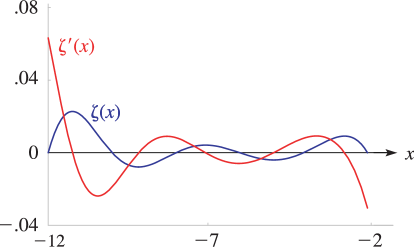
… ►With the choice

r=k

(which is crucial when

k

is large because of numerical cancellation) the integrand equals

e^{k}

at the dominant points

\theta=0,2\pi

, and in combination with the factor

k^{-k}

in front of the integral sign this gives a rough approximation to

1/k!

. … ►For additional formulas involving values of

\nabla^{2}u

and

\nabla^{4}u

on square, triangular, and cubic grids, see Collatz (1960, Table VI, pp. 542–546). …

25: 26.9 Integer Partitions: Restricted Number and Part Size

… ►

…

Figure 26.9.1: Ferrers graph of the partition

7+4+3+3+2+1

… ►The conjugate to the example in Figure 26.9.1 is

6+5+4+2+1+1+1

. … ►

Figure 26.9.2: The partition

5+5+3+2

represented as a lattice path.

… ►

p_{2}\left(n\right)=1+\left\lfloor n/2\right\rfloor,

►

p_{3}\left(n\right)=1+\left\lfloor\frac{n^{2}+6n}{12}\right\rfloor.

…

26: 25.3 Graphics

… ►

See accompanying text — Figure 25.3.2: Riemann zeta function $\zeta\left(x\right)$ and its derivative $\zeta'\left(x\right)$ , $-12\leq x\leq-2$ . Magnify

… ►

…

27: 23.19 Interrelations

… ►

23.19.1

\lambda\left(\tau\right)=16\left(\frac{{\eta}^{2}\left(2\tau\right)\eta\left(% \tfrac{1}{2}\tau\right)}{{\eta}^{3}\left(\tau\right)}\right)^{8},

ⓘ

Symbols:: $\eta\left(\NVar{\tau}\right)$ : Dedekind’s eta function (or Dedekind modular function), $\lambda\left(\NVar{\tau}\right)$ : elliptic modular function and $\tau$ : complex variable
Permalink:: http://dlmf.nist.gov/23.19.E1
Encodings:: pMML, png, TeX
See also:: Annotations for §23.19 and Ch.23

►

23.19.2

J\left(\tau\right)=\frac{4}{27}\frac{\left(1-\lambda\left(\tau\right)+{\lambda% }^{2}\left(\tau\right)\right)^{3}}{\left(\lambda\left(\tau\right)\left(1-% \lambda\left(\tau\right)\right)\right)^{2}},

ⓘ

Symbols:: $J\left(\NVar{\tau}\right)$ : Klein’s complete invariant, $\lambda\left(\NVar{\tau}\right)$ : elliptic modular function and $\tau$ : complex variable
Permalink:: http://dlmf.nist.gov/23.19.E2
Encodings:: pMML, png, TeX
See also:: Annotations for §23.19 and Ch.23

►

23.19.3

J\left(\tau\right)=\frac{{g_{2}}^{3}}{{g_{2}}^{3}-27{g_{3}}^{2}},

ⓘ

Symbols:: $J\left(\NVar{\tau}\right)$ : Klein’s complete invariant, $g_{\NVar{j}}$ : Weierstrass lattice invariants $g_{2}$ , $g_{3}$ , $\mathbb{L}$ : lattice and $\tau$ : complex variable
Permalink:: http://dlmf.nist.gov/23.19.E3
Encodings:: pMML, png, TeX
See also:: Annotations for §23.19 and Ch.23

►where

g_{2},g_{3}

are the invariants of the lattice

\mathbb{L}

with generators

1

and

\tau

; see §23.3(i). … ►

23.19.4

\Delta=(2\pi)^{12}{\eta}^{24}\left(\tau\right).

ⓘ

Symbols:: $\eta\left(\NVar{\tau}\right)$ : Dedekind’s eta function (or Dedekind modular function), $\pi$ : the ratio of the circumference of a circle to its diameter, $\Delta$ : discriminant and $\tau$ : complex variable
Referenced by:: §23.19
Permalink:: http://dlmf.nist.gov/23.19.E4
Encodings:: pMML, png, TeX
See also:: Annotations for §23.19 and Ch.23

28: 16.12 Products

… ►

16.12.1

{{}_{0}F_{1}}\left(-;a;z\right){{}_{0}F_{1}}\left(-;b;z\right)={{}_{2}F_{3}}% \left({\frac{1}{2}(a+b),\frac{1}{2}(a+b-1)\atop a,b,a+b-1};4z\right).

ⓘ

Symbols:: ${{}_{\NVar{p}}F_{\NVar{q}}}\left(\NVar{a_{1},\dots,a_{p}};\NVar{b_{1},\dots,b_% {q}};\NVar{z}\right)$ or ${{}_{\NVar{p}}F_{\NVar{q}}}\left({\NVar{a_{1},\dots,a_{p}}\atop\NVar{b_{1},% \dots,b_{q}}};\NVar{z}\right)$ : alternatively ${{}_{\NVar{p}}F_{\NVar{q}}}\left(\NVar{\mathbf{a}};\NVar{\mathbf{b}};\NVar{z}\right)$ or ${{}_{\NVar{p}}F_{\NVar{q}}}\left({\NVar{\mathbf{a}}\atop\NVar{\mathbf{b}}};% \NVar{z}\right)$
generalized hypergeometric function, $z$ : complex variable, $a,a_{1},\ldots,a_{p}$ : real or complex parameters and $b,b_{1},\ldots,b_{q}$ : real or complex parameters
Referenced by:: (10.8.3), §10.8, §10.8, §16.12, Erratum (V1.0.17) for Section 10.8
Permalink:: http://dlmf.nist.gov/16.12.E1
Encodings:: pMML, png, TeX
See also:: Annotations for §16.12 and Ch.16

… ►

16.12.2

\left({{}_{2}F_{1}}\left({a,b\atop a+b+\frac{1}{2}};z\right)\right)^{2}={{}_{3% }F_{2}}\left({2a,2b,a+b\atop a+b+\frac{1}{2},2a+2b};z\right).

ⓘ

Symbols:: ${{}_{2}F_{1}}\left(\NVar{a},\NVar{b};\NVar{c};\NVar{z}\right)$ : $=F\left(\NVar{a},\NVar{b};\NVar{c};\NVar{z}\right)$ notation for Gauss’ hypergeometric function, ${{}_{\NVar{p}}F_{\NVar{q}}}\left(\NVar{a_{1},\dots,a_{p}};\NVar{b_{1},\dots,b_% {q}};\NVar{z}\right)$ or ${{}_{\NVar{p}}F_{\NVar{q}}}\left({\NVar{a_{1},\dots,a_{p}}\atop\NVar{b_{1},% \dots,b_{q}}};\NVar{z}\right)$ : alternatively ${{}_{\NVar{p}}F_{\NVar{q}}}\left(\NVar{\mathbf{a}};\NVar{\mathbf{b}};\NVar{z}\right)$ or ${{}_{\NVar{p}}F_{\NVar{q}}}\left({\NVar{\mathbf{a}}\atop\NVar{\mathbf{b}}};% \NVar{z}\right)$
generalized hypergeometric function, $z$ : complex variable, $a,a_{1},\ldots,a_{p}$ : real or complex parameters and $b,b_{1},\ldots,b_{q}$ : real or complex parameters
Referenced by:: §16.12, §17.9(iii), Erratum (V1.1.12) for Subsection 17.9(iii)
Permalink:: http://dlmf.nist.gov/16.12.E2
Encodings:: pMML, png, TeX
See also:: Annotations for §16.12 and Ch.16

… ►

16.12.3

\left({{}_{2}F_{1}}\left({a,b\atop c};z\right)\right)^{2}=\sum_{k=0}^{\infty}% \frac{{\left(2a\right)_{k}}{\left(2b\right)_{k}}{\left(c-\frac{1}{2}\right)_{k% }}}{{\left(c\right)_{k}}{\left(2c-1\right)_{k}}k!}{{}_{4}F_{3}}\left({-\frac{1% }{2}k,\frac{1}{2}(1-k),a+b-c+\frac{1}{2},\frac{1}{2}\atop a+\frac{1}{2},b+% \frac{1}{2},\frac{3}{2}-k-c};1\right)z^{k},

|z|<1

ⓘ

Symbols:: ${{}_{2}F_{1}}\left(\NVar{a},\NVar{b};\NVar{c};\NVar{z}\right)$ : $=F\left(\NVar{a},\NVar{b};\NVar{c};\NVar{z}\right)$ notation for Gauss’ hypergeometric function, ${{}_{\NVar{p}}F_{\NVar{q}}}\left(\NVar{a_{1},\dots,a_{p}};\NVar{b_{1},\dots,b_% {q}};\NVar{z}\right)$ or ${{}_{\NVar{p}}F_{\NVar{q}}}\left({\NVar{a_{1},\dots,a_{p}}\atop\NVar{b_{1},% \dots,b_{q}}};\NVar{z}\right)$ : alternatively ${{}_{\NVar{p}}F_{\NVar{q}}}\left(\NVar{\mathbf{a}};\NVar{\mathbf{b}};\NVar{z}\right)$ or ${{}_{\NVar{p}}F_{\NVar{q}}}\left({\NVar{\mathbf{a}}\atop\NVar{\mathbf{b}}};% \NVar{z}\right)$
generalized hypergeometric function, ${\left(\NVar{a}\right)_{\NVar{n}}}$ : Pochhammer’s symbol (or shifted factorial), $!$ : factorial (as in $n!$ ), $z$ : complex variable, $a,a_{1},\ldots,a_{p}$ : real or complex parameters and $b,b_{1},\ldots,b_{q}$ : real or complex parameters
Referenced by:: §16.12
Permalink:: http://dlmf.nist.gov/16.12.E3
Encodings:: pMML, png, TeX
See also:: Annotations for §16.12 and Ch.16

…

29: 13.22 Zeros

… ►From (13.14.2) and (13.14.3)

M_{\kappa,\mu}\left(z\right)

has the same zeros as

M\left(\tfrac{1}{2}+\mu-\kappa,1+2\mu,z\right)

and

W_{\kappa,\mu}\left(z\right)

has the same zeros as

U\left(\tfrac{1}{2}+\mu-\kappa,1+2\mu,z\right)

, hence the results given in §13.9 can be adopted. … ►

13.22.1

\phi_{r}=\frac{j_{2\mu,r}^{2}}{4\kappa}+j_{2\mu,r}O\left(\kappa^{-\frac{3}{2}}% \right),

ⓘ

Symbols:: $O\left(\NVar{x}\right)$ : order not exceeding, $\phi_{r}$ : positive zeros and $j_{b,r}$ : positive zero of Bessel
Referenced by:: §13.22, §13.22
Permalink:: http://dlmf.nist.gov/13.22.E1
Encodings:: pMML, png, TeX
See also:: Annotations for §13.22 and Ch.13

►where

j_{2\mu,r}

is the

r

th positive zero of the Bessel function

J_{2\mu}\left(x\right)

(§10.21(i)). …

30: 25.20 Approximations

… ►

•

Piessens and Branders (1972) gives the coefficients of the Chebyshev-series expansions of $s\zeta\left(s+1\right)$ and $\zeta\left(s+k\right)$ , $k=2,3,4,5,8$ , for $0\leq s\leq 1$ (23D).

►

•

Luke (1969b, p. 306) gives coefficients in Chebyshev-series expansions that cover $\zeta\left(s\right)$ for $0\leq s\leq 1$ (15D), $\zeta\left(s+1\right)$ for $0\leq s\leq 1$ (20D), and $\ln\xi\left(\tfrac{1}{2}+ix\right)$ (§25.4) for $-1\leq x\leq 1$ (20D). For errata see Piessens and Branders (1972).

►

•

Morris (1979) gives rational approximations for $\operatorname{Li}_{2}\left(x\right)$ (§25.12(i)) for $0.5\leq x\leq 1$ . Precision is varied with a maximum of 24S.

►

•

Antia (1993) gives minimax rational approximations for $\Gamma\left(s+1\right)F_{s}(x)$ , where $F_{s}(x)$ is the Fermi–Dirac integral (25.12.14), for the intervals $-\infty<x\leq 2$ and $2\leq x<\infty$ , with $s=-\frac{1}{2},\frac{1}{2},\frac{3}{2},\frac{5}{2}$ . For each $s$ there are three sets of approximations, with relative maximum errors $10^{-4},10^{-8},10^{-12}$ .