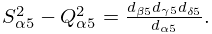
§19.29 Reduction of General Elliptic Integrals
Contents
§19.29(i) Reduction Theorems
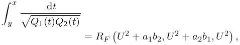
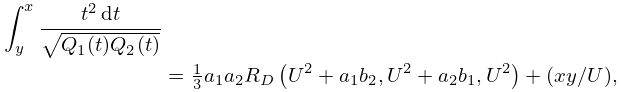
These theorems reduce integrals over a real interval of certain integrands containing the square root of a quartic or cubic polynomial to symmetric integrals over containing the square root of a cubic polynomial (compare §19.16(i)). Let
| 19.29.1 | ||||
| , , | ||||
| 19.29.2 | |||
| if , | |||
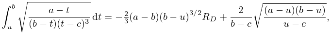
and assume that the line segment with endpoints and lies in for . If
| 19.29.3 | |||
and is any permutation of the numbers , then
| 19.29.4 | |||
where
| 19.29.5 | ||||
There are only three distinct ’s with subscripts , and at most one of them can be 0 because the ’s are nonzero. Then
| 19.29.6 | ||||
| , | ||||
| . | ||||
| 19.29.7 | |||
| . | |||
| 19.29.8 | |||
| , | |||
where
| 19.29.9 | ||||
The Cauchy principal value is taken when or is real and negative. Cubic cases of these formulas are obtained by setting one of the factors in (19.29.3) equal to 1.
The advantages of symmetric integrals for tables of integrals and symbolic integration are illustrated by (19.29.4) and its cubic case, which replace the formulas in Gradshteyn and Ryzhik (2000, 3.147, 3.131, 3.152) after taking as the variable of integration in 3.152. Moreover, the requirement that one limit of integration be a branch point of the integrand is eliminated without doubling the number of standard integrals in the result. (19.29.7) subsumes all 72 formulas in Gradshteyn and Ryzhik (2000, 3.168), and its cubic cases similarly replace the formulas in Gradshteyn and Ryzhik (2000, 3.133, 3.142, and 3.141(1-18)). For example, 3.142(2) is included as
| 19.29.10 | |||
| , | |||
where the arguments of the function are, in order, , , .
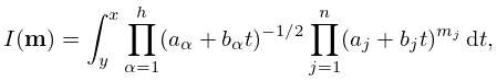
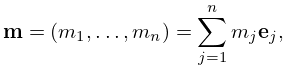
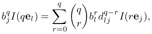
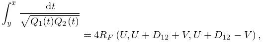
§19.29(ii) Reduction to Basic Integrals
(19.2.3) can be written
| 19.29.11 | |||
where , or 4, , and is an integer. Define
| 19.29.12 | |||
where is an -tuple with 1 in the th position and 0’s elsewhere. Define also and retain the notation and conditions associated with (19.29.1) and (19.29.2). The integrals in (19.29.4), (19.29.7), and (19.29.8) are , , and , respectively.
The only cases of that are integrals of the first kind are the two ( or 4) with . The only cases that are integrals of the third kind are those in which at least one with is a negative integer and those in which and is a positive integer. All other cases are integrals of the second kind.
can be reduced to a linear combination of basic integrals and algebraic functions. In the cubic case () the basic integrals are
| 19.29.13 | |||
| . | |||
In the quartic case () the basic integrals are
| 19.29.14 | |||
| ; | |||
| . | |||
Basic integrals of type , , are not linearly independent, nor are those of type , .
The reduction of is carried out by a relation derived from partial fractions and by use of two recurrence relations. These are given in Carlson (1999, (2.19), (3.5), (3.11)) and simplified in Carlson (2002, (1.10), (1.7), (1.8)) by means of modified definitions. Partial fractions provide a reduction to integrals in which has at most one nonzero component, and these are then reduced to basic integrals by the recurrence relations. A special case of Carlson (1999, (2.19)) is given by
| 19.29.15 | |||
| , | |||
which shows how to express the basic integral in terms of symmetric integrals by using (19.29.4) and either (19.29.7) or (19.29.8). The first choice gives a formula that includes the 18+9+18 = 45 formulas in Gradshteyn and Ryzhik (2000, 3.133, 3.156, 3.158), and the second choice includes the 8+8+8+12 = 36 formulas in Gradshteyn and Ryzhik (2000, 3.151, 3.149, 3.137, 3.157) (after setting in some cases).
If , then the recurrence relation (Carlson (1999, (3.5))) has the special case
| 19.29.16 | |||
where is any permutation of the numbers , and
| 19.29.17 | |||
(This shows why is not needed as a basic integral in the cubic case.) In the quartic case this recurrence relation has an extra term in , and hence , , is a basic integral. It can be expressed in terms of symmetric integrals by setting and in (19.29.8).
The other recurrence relation is
| 19.29.18 | |||
| ; | |||
see Carlson (1999, (3.11)). An example that uses (19.29.15)–(19.29.18) is given in §19.34.
For an implementation by James FitzSimons of the method for reducing to basic integrals and extensive tables of such reductions, see Carlson (1999) and Carlson and FitzSimons (2000).
Another method of reduction is given in Gray (2002). It depends primarily on multivariate recurrence relations that replace one integral by two or more.
§19.29(iii) Examples
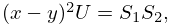
The first formula replaces (19.14.4)–(19.14.10). Define , , and assume both ’s are positive for . Then
| 19.29.19 | |||
| 19.29.20 | |||
and
| 19.29.21 | |||
where
| 19.29.22 | |||
If both square roots in (19.29.22) are 0, then the indeterminacy in the two preceding equations can be removed by using (19.27.8) to evaluate the integral as multiplied either by or by in the cases of (19.29.20) or (19.29.21), respectively. If , then is found by taking the limit. For example,
| 19.29.23 | |||
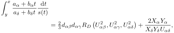
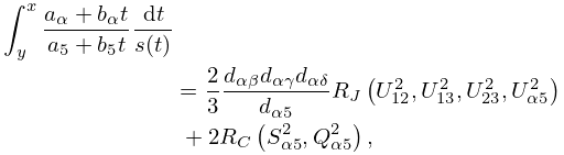
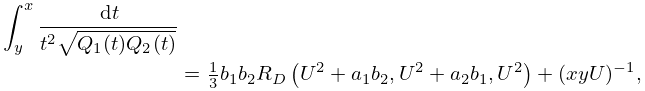
Next, for , define , and assume both ’s are positive for . If each has real zeros, then (19.29.4) may be simpler than
| 19.29.24 | |||
where
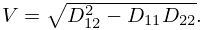
| 19.29.25 | ||||
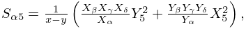
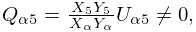
(The variables of are real and nonnegative unless both ’s have real zeros and those of interlace those of .) If , where both linear factors are positive for , and , then (19.29.25) is modified so that
| 19.29.26 | ||||
with other quantities remaining as in (19.29.25). In the cubic case, in which , , (19.29.26) reduces further to
| 19.29.27 | ||||
For example, because , we find that when
| 19.29.28 | |||
where
| 19.29.29 | ||||
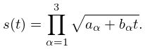
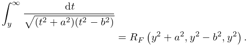
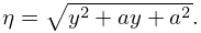
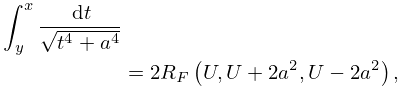
Lastly, define and assume is positive and monotonic for . Then
| 19.29.30 | |||
where
| 19.29.31 | |||
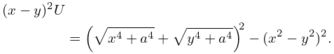
For example, if and , then
| 19.29.32 | |||
where
| 19.29.33 | |||
