Mellin transform with respect to lattice parameter

SearchAdvancedHelp

(0.004 seconds)

21—30 of 910 matching pages

21: 12.16 Mathematical Applications

… ►PCFs are also used in integral transforms with respect to the parameter, and inversion formulas exist for kernels containing PCFs. …Integral transforms and sampling expansions are considered in Jerri (1982).

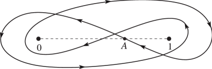
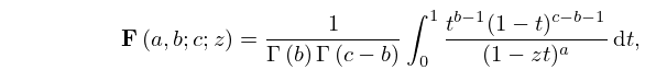
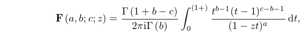
22: 15.6 Integral Representations

§15.6 Integral Representations

… ►

15.6.1 $$𝐅(a,b;c;z)=\frac{1}{\mathrm{\Gamma }\left(b\right)\mathrm{\Gamma }\left(c-b\right)}{\int }_0^1\frac{t^{b-1}{(1-t)}^{c-b-1}}{{(1-zt)}^a}dt,$$ ; $\mathrm{\Re }c>\mathrm{\Re }b>0$.

ⓘ

Symbols:

$\mathrm{\Gamma }\left(z\right)$: gamma function, $\pi$: the ratio of the circumference of a circle to its diameter, $dx$: differential of $x$ , $\int$: integral, $\mathrm{ph}$: phase, $\mathrm{\Re }$: real part, $𝐅(a,b;c;z)$ or $𝐅(\genfrac{}{}{0pt}{}{a,b}{c};z)$: $={}_2{}^{}𝐅_1^{}(a,b;c;z)$ Olver’s hypergeometric function, $z$: complex variable, $a$: real or complex parameter, $b$: real or complex parameter and $c$: real or complex parameter

Keywords:

Mellintransform

Referenced by:

§15.19(iii), (15.4.34), §15.6, §15.6, Erratum (V1.0.23) for Equations (15.6.1)–(15.6.9), Erratum (V1.0.23) for Equations (15.6.1)–(15.6.9)

Permalink:

http://dlmf.nist.gov/15.6.E1

Encodings:

pMML, png, TeX

Addition (effective with 1.0.23):

The Olver hypergeometric function $𝐅(a,b;c;z)$, previously omitted from the left-hand side to make the formula more concise, has been added. The constraint , originally mentioned in the text, has been directly added to the formula.

See also:

Annotations for §15.6 and Ch.15

►

15.6.2 $$𝐅(a,b;c;z)=\frac{\mathrm{\Gamma }\left(1+b-c\right)}{2\pi \mathrm{i}\mathrm{\Gamma }\left(b\right)}{\int }_0^{(1+)}\frac{t^{b-1}{(t-1)}^{c-b-1}}{{(1-zt)}^a}dt,$$ ; $c-b\ne 1,2,3,\mathrm{\dots }$, $\mathrm{\Re }b>0$.

ⓘ

Symbols:

$\mathrm{\Gamma }\left(z\right)$: gamma function, $\pi$: the ratio of the circumference of a circle to its diameter, $dx$: differential of $x$ , $\mathrm{i}$: imaginary unit, $\int$: integral, $\mathrm{ph}$: phase, $\mathrm{\Re }$: real part, $𝐅(a,b;c;z)$ or $𝐅(\genfrac{}{}{0pt}{}{a,b}{c};z)$: $={}_2{}^{}𝐅_1^{}(a,b;c;z)$ Olver’s hypergeometric function, $z$: complex variable, $a$: real or complex parameter, $b$: real or complex parameter and $c$: real or complex parameter

Keywords:

Mellintransform

Referenced by:

§15.6

Permalink:

http://dlmf.nist.gov/15.6.E2

Encodings:

pMML, png, TeX

Addition (effective with 1.0.23):

The Olver hypergeometric function $𝐅(a,b;c;z)$, previously omitted from the left-hand side to make the formula more concise, has been added. The constraint , originally mentioned in the text, has been directly added to the formula.

See also:

Annotations for §15.6 and Ch.15

… ►However, this reverses the direction of the integration contour, and in consequence (15.6.5) would need to be multiplied by $-1$. … ►

►►

Figure 15.6.1: $t$-plane. … Magnify

23: 10.43 Integrals

… ►

§10.43(v) Kontorovich–Lebedev Transform

►The Kontorovich–Lebedev transform of a function $g(x)$ is defined as … ►For asymptotic expansions of the direct transform (10.43.30) see Wong (1981), and for asymptotic expansions of the inverse transform (10.43.31) see Naylor (1990, 1996). ►For collections of the Kontorovich–Lebedev transform, see Erdélyi et al. (1954b, Chapter 12), Prudnikov et al. (1986b, pp. 404–412), and Oberhettinger (1972, Chapter 5). … ►For collections of integrals of the functions $I_{\nu }\left(z\right)$ and $K_{\nu }\left(z\right)$, including integrals with respect to the order, see Apelblat (1983, §12), Erdélyi et al. (1953b, §§7.7.1–7.7.7 and 7.14–7.14.2), Erdélyi et al. (1954a, b), Gradshteyn and Ryzhik (2000, §§5.5, 6.5–6.7), Gröbner and Hofreiter (1950, pp. 197–203), Luke (1962), Magnus et al. (1966, §3.8), Marichev (1983, pp. 191–216), Oberhettinger (1972), Oberhettinger (1974, §§1.11 and 2.7), Oberhettinger (1990, §§1.17–1.20 and 2.17–2.20), Oberhettinger and Badii (1973, §§1.15 and 2.13), Okui (1974, 1975), Prudnikov et al. (1986b, §§1.11–1.12, 2.15–2.16, 3.2.8–3.2.10, and 3.4.1), Prudnikov et al. (1992a, §§3.15, 3.16), Prudnikov et al. (1992b, §§3.15, 3.16), Watson (1944, Chapter 13), and Wheelon (1968).

24: Bibliography S

… ►

The Laplace Transform: Theory and Applications. Undergraduate Texts in Mathematics, Springer-Verlag, New York.

ⓘ

External Links:

ISBN 0-387-98698-7, MathReview (Philip Heywood), ZentralBlatt

Referenced by:

§1.14(iii), §1.14(vii).

Encodings:

BibTeX

… ►

Numerical evaluation of spherical Bessel transforms via fast Fourier transforms. J. Comput. Phys. 100 (2), pp. 294–296.

ⓘ

External Links:

ISSN 0021-9991, Document, MathReview, ZentralBlatt

Referenced by:

§10.74(vii).

Encodings:

BibTeX

… ►

Asymptotic expansions of Mellin transforms and analogues of Watson’s lemma. SIAM J. Math. Anal. 16 (4), pp. 896–906.

ⓘ

External Links:

ISSN 0036-1410, Document, Link, MathReview (John S. Lew), ZentralBlatt

Referenced by:

§2.3(vi).

Encodings:

BibTeX

… ►

Asymptotic expansion of Mellin transforms in the complex plane. Int. J. Pure Appl. Math. 71 (3), pp. 465–480.

ⓘ

External Links:

ISSN 1311-8080, MathReview Entry, ZentralBlatt

Referenced by:

§2.3(vi).

Encodings:

BibTeX

… ►

A Guide to Distribution Theory and Fourier Transforms. Studies in Advanced Mathematics, CRC Press, Boca Raton, FL.

ⓘ

External Links:

ISBN 0-8493-8273-4, MathReview (J. Horváth), ZentralBlatt

Referenced by:

§18.17(v).

Encodings:

BibTeX

…

25: Bibliography P

… ►

On two-sided estimates, uniform with respect to the real argument and index, for modified Bessel functions. Mat. Zametki 65 (5), pp. 681–692 (Russian).

ⓘ

Notes:

English translation in Math. Notes 65 (1999) pp. 571-581.

External Links:

ISSN 0025-567X, Document, MathReview (Boro Döring), ZentralBlatt

Referenced by:

§10.37.

Encodings:

BibTeX

… ►

Asymptotics and Mellin-Barnes Integrals. Cambridge University Press, Cambridge.

ⓘ

External Links:

ISBN 0-521-79001-8, MathReview, ZentralBlatt

Referenced by:

§1.14(iv), §10.32(iii), §10.32(ii), §10.46, §10.9(iii), §10.9(ii), §16.11(i), §16.11(ii), §2.10(iii), §2.11(iii), §2.11(v), §2.5(ii), §2.5(ii), Ch.2, §24.7(ii), §25.9, §5.11(ii), §5.11(iii), §5.13, §5.19(ii), §5.6(ii), Ch.5, §8.6(ii), Profile Richard B. Paris.

Encodings:

BibTeX

… ►

Smoothing of the Stokes phenomenon using Mellin-Barnes integrals. J. Comput. Appl. Math. 41 (1-2), pp. 117–133.

ⓘ

External Links:

ISSN 0377-0427, Document, MathReview (Anatoly Kilbas), ZentralBlatt

Referenced by:

§2.11(v).

Encodings:

BibTeX

… ►

Bounds for ratios of modified Bessel functions. Integral Transform. Spec. Funct. 9 (4), pp. 293–298.

ⓘ

External Links:

ISSN 1065-2469, Document, MathReview, ZentralBlatt

Referenced by:

§10.37.

Encodings:

BibTeX

… ►

Fourier Series and Integral Transforms. Cambridge University Press, Cambridge.

ⓘ

External Links:

ISBN 0-521-59209-7; 0-521-59771-4, MathReview, ZentralBlatt

Referenced by:

§1.14(vii).

Encodings:

BibTeX

…

26: 16.5 Integral Representations and Integrals

… ►Suppose first that $L$ is a contour that starts at infinity on a line parallel to the positive real axis, encircles the nonnegative integers in the negative sense, and ends at infinity on another line parallel to the positive real axis. … ►Secondly, suppose that $L$ is a contour from $-\mathrm{i}\mathrm{\infty }$ to $\mathrm{i}\mathrm{\infty }$. … ►Lastly, the restrictions on the parameters can be eased by replacing the integration paths with loop contours; see Luke (1969a, §3.6). ►Laplace transforms and inverse Laplace transforms of generalized hypergeometric functions are given in Prudnikov et al. (1992a, §3.38) and Prudnikov et al. (1992b, §3.36). …

27: 10.22 Integrals

… ►

§10.22(v) Hankel Transform

►The Hankel transform (or Bessel transform) of a function $f(x)$ is defined as … ►For collections of Hankel transforms see Erdélyi et al. (1954b, Chapter 8) and Oberhettinger (1972). ►The following two formulas are generalizations of the Hankel transform. …This is the Weber transform. …

28: Errata

… ►The specific updates to Chapter 18 include some results for general orthogonal polynomials including quadratic transformations, uniqueness of orthogonality measure and completeness, moments, continued fractions, and some special classes of orthogonal polynomials. … ►

The Weierstrass lattice roots $e_j,$ were linked inadvertently as the base of the natural logarithm. In order to resolve this inconsistency, the lattice roots $e_j$, and lattice invariants $g_2$, $g_3$, now link to their respective definitions (see §§23.2(i), 23.3(i)).

Reported by Felix Ospald.

… ►

The descriptions for the paths of integration of the Mellin-Barnes integrals (8.6.10)–(8.6.12) have been updated. The description for (8.6.11) now states that the path of integration is to the right of all poles. Previously it stated incorrectly that the path of integration had to separate the poles of the gamma function from the pole at $s=0$. The paths of integration for (8.6.10) and (8.6.12) have been clarified. In the case of (8.6.10), it separates the poles of the gamma function from the pole at $s=a$ for $\gamma (a,z)$. In the case of (8.6.12), it separates the poles of the gamma function from the poles at $s=0,1,2,\mathrm{\dots }$.

Reported 2017-07-10 by Kurt Fischer.

… ►

There have been extensive changes in the notation used for the integral transforms defined in §1.14. These changes are applied throughout the DLMF. The following table summarizes the changes.

Transform	New	Abbreviated	Old
	Notation	Notation	Notation
Fourier	$ℱ\left(f\right)\left(x\right)$	$ℱf\left(x\right)$
Fourier Cosine	${ℱ}_c\left(f\right)\left(x\right)$	${ℱ}_{c}f\left(x\right)$
Fourier Sine	${ℱ}_s\left(f\right)\left(x\right)$	${ℱ}_{s}f\left(x\right)$
Laplace	$ℒ\left(f\right)\left(s\right)$	$ℒf\left(s\right)$	$ℒ(f(t);s)$
Mellin	$ℳ\left(f\right)\left(s\right)$	$ℳf\left(s\right)$	$ℳ(f;s)$
Hilbert	$\mathscr{H}\left(f\right)\left(s\right)$	$\mathscr{H}f\left(s\right)$	$\mathscr{H}(f;s)$
Stieltjes	$𝒮\left(f\right)\left(s\right)$	$𝒮f\left(s\right)$	$𝒮(f;s)$

Previously, for the Fourier, Fourier cosine and Fourier sine transforms, either temporary local notations were used or the Fourier integrals were written out explicitly.

… ►

The title was changed from Transformations of Higher ${}_r{}^{}\varphi _r^{}$ Functions to Further Transformations of ${}_{r+1}{}^{}\varphi _r^{}$ Functions.

…

29: 14.17 Integrals

… ►

14.17.7 $${\int }_{-1}^1{𝖯}_l^m\left(x\right){𝖯}_n^{-m}\left(x\right)dx=\frac{{(-1)}^m}{l+\frac{1}{2}}{\delta }_{l,n},$$

ⓘ

Symbols:

: Ferrers function of the first kind, ${\delta }_{j,k}$: Kronecker delta, $dx$: differential of $x$ , $\int$: integral, $x$: real variable, $m$: nonnegative integer, $n$: nonnegative integer and $l$: nonnegative integer

Referenced by:

§14.17(iii)

Permalink:

http://dlmf.nist.gov/14.17.E7

Encodings:

pMML, png, TeX

Clarification (effective with 1.0.17):

The Kronecker delta symbol has been moved furthest to the right and ${(-1)}^m$ has been moved to the numerator of the fraction.

See also:

Annotations for §14.17(iii), §14.17 and Ch.14

… ►

§14.17(v) Laplace Transforms

►For Laplace transforms and inverse Laplace transforms involving associated Legendre functions, see Erdélyi et al. (1954a, pp. 179–181, 270–272), Oberhettinger and Badii (1973, pp. 113–118, 317–324), Prudnikov et al. (1992a, §§3.22, 3.32, and 3.33), and Prudnikov et al. (1992b, §§3.20, 3.30, and 3.31). ►

§14.17(vi) Mellin Transforms

►For Mellin transforms involving associated Legendre functions see Oberhettinger (1974, pp. 69–82) and Marichev (1983, pp. 247–283), and for inverse transforms see Oberhettinger (1974, pp. 205–215).

30: 12.5 Integral Representations

… ►

12.5.4 $$U(a,z)=\sqrt{\frac{2}{\pi }}{\mathrm{e}}^{\frac{1}{4}{z}^2}{\int }_0^{\mathrm{\infty }}{t}^{-a-\frac{1}{2}}{\mathrm{e}}^{-\frac{1}{2}{t}^2}\cos \left(zt+\left(\frac{1}{2}a+\frac{1}{4}\right)\pi \right)dt,$$ .

ⓘ

Symbols:

$\pi$: the ratio of the circumference of a circle to its diameter, $\cos z$: cosine function, $dx$: differential of $x$ , $\mathrm{e}$: base of natural logarithm, $\int$: integral, $U(a,z)$: parabolic cylinder function, $\mathrm{\Re }$: real part, $z$: complex variable and $a$: real or complex parameter

Referenced by:

§12.5(i)

Permalink:

http://dlmf.nist.gov/12.5.E4

Encodings:

pMML, png, TeX

See also:

Annotations for §12.5(i), §12.5 and Ch.12

… ►The following integrals correspond to those of §12.5(i). … ►

§12.5(iii) Mellin–Barnes Integrals

►

12.5.8 $$U(a,z)=\frac{{\mathrm{e}}^{-\frac{1}{4}{z}^2}{z}^{-a-\frac{1}{2}}}{2\pi \mathrm{i}\mathrm{\Gamma }\left(\frac{1}{2}+a\right)}{\int }_{-\mathrm{i}\mathrm{\infty }}^{\mathrm{i}\mathrm{\infty }}\mathrm{\Gamma }\left(t\right)\mathrm{\Gamma }\left(\frac{1}{2}+a-2t\right)2^t{z}^{2t}dt,$$ $a\ne -\frac{1}{2},-\frac{3}{2},-\frac{5}{2},\mathrm{\dots }$, ,

ⓘ

Symbols:

$\mathrm{\Gamma }\left(z\right)$: gamma function, $\pi$: the ratio of the circumference of a circle to its diameter, $dx$: differential of $x$ , $\mathrm{e}$: base of natural logarithm, $\mathrm{i}$: imaginary unit, $\int$: integral, $U(a,z)$: parabolic cylinder function, $\mathrm{ph}$: phase, $z$: complex variable and $a$: real or complex parameter

Keywords:

Mellintransform

A&S Ref:

19.5.13 (modification and correction of)

Referenced by:

§12.5(iii)

Permalink:

http://dlmf.nist.gov/12.5.E8

Encodings:

pMML, png, TeX

See also:

Annotations for §12.5(iii), §12.5 and Ch.12

… ►

12.5.9 $$V(a,z)=\sqrt{\frac{2}{\pi }}\frac{{\mathrm{e}}^{\frac{1}{4}{z}^2}{z}^{a-\frac{1}{2}}}{2\pi \mathrm{i}\mathrm{\Gamma }\left(\frac{1}{2}-a\right)}{\int }_{-\mathrm{i}\mathrm{\infty }}^{\mathrm{i}\mathrm{\infty }}\mathrm{\Gamma }\left(t\right)\mathrm{\Gamma }\left(\frac{1}{2}-a-2t\right)2^t{z}^{2t}\cos \left(\pi t\right)dt,$$ $a\ne \frac{1}{2},\frac{3}{2},\frac{5}{2},\mathrm{\dots }$, ,

ⓘ

Symbols:

$\mathrm{\Gamma }\left(z\right)$: gamma function, $\pi$: the ratio of the circumference of a circle to its diameter, $\cos z$: cosine function, $dx$: differential of $x$ , $\mathrm{e}$: base of natural logarithm, $\mathrm{i}$: imaginary unit, $\int$: integral, $V(a,z)$: parabolic cylinder function, $\mathrm{ph}$: phase, $z$: complex variable and $a$: real or complex parameter

Keywords:

Mellintransform

A&S Ref:

19.5.13 (modification and correction of)

Referenced by:

§12.5(iii), §12.8(ii)

Permalink:

http://dlmf.nist.gov/12.5.E9

Encodings:

pMML, png, TeX

See also:

Annotations for §12.5(iii), §12.5 and Ch.12

…