§2.11 Remainder Terms; Stokes Phenomenon

Permalink:: http://dlmf.nist.gov/2.11

§2.11(i) Numerical Use of Asymptotic Expansions
§2.11(ii) Connection Formulas
§2.11(iii) Exponentially-Improved Expansions
§2.11(iv) Stokes Phenomenon
§2.11(v) Exponentially-Improved Expansions (continued)
§2.11(vi) Direct Numerical Transformations

§2.11(i) Numerical Use of Asymptotic Expansions

Notes:: See Olver (1997b, pp. 76–78).
Keywords:: asymptotic approximations and expansions
Referenced by:: §2.11(ii)
Permalink:: http://dlmf.nist.gov/2.11.i

When a rigorous bound or reliable estimate for the remainder term is unavailable, it is unsafe to judge the accuracy of an asymptotic expansion merely from the numerical rate of decrease of the terms at the point of truncation. Even when the series converges this is unwise: the tail needs to be majorized rigorously before the result can be guaranteed. For divergent expansions the situation is even more difficult. First, it is impossible to bound the tail by majorizing its terms. Secondly, the asymptotic series represents an infinite class of functions, and the remainder depends on which member we have in mind.

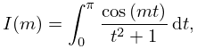
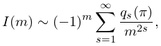
As an example consider

2.11.1 $I(m)=\int _{{0}}^{{\pi}}\frac{\mathop{\cos\/}\nolimits\!\left(mt\right)}{t^{2}+1}dt,$

Symbols:: $\mathop{\cos\/}\nolimits z$ : cosine function, $dx$ : differential of $x$ , $\int$ : integral and $I(m)$ : integral
Permalink:: http://dlmf.nist.gov/2.11.E1
Encodings:: TeX, pMML, png

with $m$ a large integer. By integration by parts (§2.3(i))

2.11.2 $I(m)\sim(-1)^{m}\sum _{{s=1}}^{{\infty}}\frac{q_{s}(\pi)}{m^{{2s}}},$ $m\to\infty$ ,

Symbols:: $\sim$ : asymptotic equality, $I(m)$ : integral and $q_{s}(t)$ : coefficients
Referenced by:: §2.11(i)
Permalink:: http://dlmf.nist.gov/2.11.E2
Encodings:: TeX, pMML, png

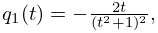
with

2.11.3

$q_{1}(t)=-\frac{2t}{(t^{2}+1)^{2}},$

$q_{2}(t)=\frac{24(t^{3}-t)}{(t^{2}+1)^{4}},$

$q_{3}(t)=-\frac{240(3t^{5}-10t^{3}+3t)}{(t^{2}+1)^{6}}.$

Symbols:: $q_{s}(t)$ : coefficients
Permalink:: http://dlmf.nist.gov/2.11.E3
Encodings:: TeX, TeX, TeX, pMML, pMML, pMML, png, png, png

On rounding to 5D, we have $q_{1}(\pi)=-0.05318$ , $q_{2}(\pi)=0.04791$ , $q_{3}(\pi)=-0.08985$ . Hence

2.11.4 $I(10)\sim-0.00053\; 18+0.00000\; 48-0.00000\; 0 1=-0.00052\; 71.$

Symbols:: $\sim$ : asymptotic equality and $I(m)$ : integral
Referenced by:: §2.11(i)
Permalink:: http://dlmf.nist.gov/2.11.E4
Encodings:: TeX, pMML, png

But this answer is incorrect: to 7D $I(10)=-0.00045\; 58$ . The error term is, in fact, approximately 700 times the last term obtained in (2.11.4). The explanation is that (2.11.2) is a more accurate expansion for the function $I(m)-\frac{1}{2}\pi e^{{-m}}$ than it is for $I(m)$ ; see Olver (1997b, pp. 76–78).

In order to guard against this kind of error remaining undetected, the wanted function may need to be computed by another method (preferably nonasymptotic) for the smallest value of the (large) asymptotic variable $x$ that is intended to be used. If the results agree within $S$ significant figures, then it is likely—but not certain—that the truncated asymptotic series will yield at least $S$ correct significant figures for larger values of $x$ . For further discussion see Bosley (1996).

In $\Complex$ both the modulus and phase of the asymptotic variable $z$ need to be taken into account. Suppose an asymptotic expansion holds as $z\to\infty$ in any closed sector within $\alpha<\mathop{\mathrm{ph}\/}\nolimits z<\beta$ , say, but not in $\alpha\leq\mathop{\mathrm{ph}\/}\nolimits z\leq\beta$ . Then numerical accuracy will disintegrate as the boundary rays $\mathop{\mathrm{ph}\/}\nolimits z=\alpha$ , $\mathop{\mathrm{ph}\/}\nolimits z=\beta$ are approached. In consequence, practical application needs to be confined to a sector $\alpha^{{\prime}}\leq\mathop{\mathrm{ph}\/}\nolimits z\leq\beta^{{\prime}}$ well within the sector of validity, and independent evaluations carried out on the boundaries for the smallest value of $|z|$ intended to be used. The choice of $\alpha^{{\prime}}$ and $\beta^{{\prime}}$ is facilitated by a knowledge of the relevant Stokes lines; see §2.11(iv) below.

However, regardless whether we can bound the remainder, the accuracy achievable by direct numerical summation of a divergent asymptotic series is always limited. The rest of this section is devoted to general methods for increasing this accuracy.

§2.11(ii) Connection Formulas

Keywords:: asymptotic approximations and expansions, generalized exponential integral
Referenced by:: §2.11(iii), §6.12(i), §7.12(i), §8.20(i), §8.22(i)
Permalink:: http://dlmf.nist.gov/2.11.ii

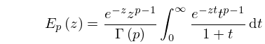
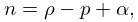
From §8.19(i) the generalized exponential integral is given by

2.11.5 $\mathop{E_{{p}}\/}\nolimits\!\left(z\right)=\frac{e^{{-z}}z^{{p-1}}}{\mathop{\Gamma\/}\nolimits\!\left(p\right)}\int _{{0}}^{{\infty}}\frac{e^{{-zt}}t^{{p-1}}}{1+t}dt$

Symbols:: $\mathop{\Gamma\/}\nolimits\!\left(z\right)$ : gamma function, $dx$ : differential of $x$ , $e$ : base of exponential function, $\mathop{E_{{p}}\/}\nolimits\!\left(z\right)$ : generalized exponential integral and $\int$ : integral
Referenced by:: §2.11(iii)
Permalink:: http://dlmf.nist.gov/2.11.E5
Encodings:: TeX, pMML, png

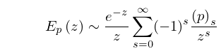
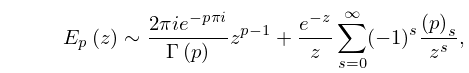
when $\realpart{p}>0$ and $|\mathop{\mathrm{ph}\/}\nolimits z|<\frac{1}{2}\pi$ , and by analytic continuation for other values of $p$ and $z$ . Application of Watson’s lemma (§2.4(i)) yields

2.11.6 $\mathop{E_{{p}}\/}\nolimits\!\left(z\right)\sim\frac{e^{{-z}}}{z}\sum _{{s=0}}^{{\infty}}(-1)^{s}\frac{\left(p\right)_{{s}}}{z^{s}}$

Symbols:: $\left(a\right)_{{n}}$ : Pochhammer’s symbol, $e$ : base of exponential function, $\mathop{E_{{p}}\/}\nolimits\!\left(z\right)$ : generalized exponential integral and $\sim$ : asymptotic equality
Referenced by:: §2.11(ii), §2.11(iii), §2.11(iii), §2.11(iv), §2.11(iv)
Permalink:: http://dlmf.nist.gov/2.11.E6
Encodings:: TeX, pMML, png

when $p$ is fixed and $z\to\infty$ in any closed sector within $|\mathop{\mathrm{ph}\/}\nolimits z|<\frac{3}{2}\pi$ . As noted in §2.11(i), poor accuracy is yielded by this expansion as $\mathop{\mathrm{ph}\/}\nolimits z$ approaches $\frac{3}{2}\pi$ or $-\frac{3}{2}\pi$ . However, on combining (2.11.6) with the connection formula (8.19.18), with $m=1$ , we derive

2.11.7 $\mathop{E_{{p}}\/}\nolimits\!\left(z\right)\sim\frac{2\pi ie^{{-p\pi i}}}{\mathop{\Gamma\/}\nolimits\!\left(p\right)}z^{{p-1}}+\frac{e^{{-z}}}{z}\sum _{{s=0}}^{{\infty}}(-1)^{s}\frac{\left(p\right)_{{s}}}{z^{s}},$

Symbols:: $\mathop{\Gamma\/}\nolimits\!\left(z\right)$ : gamma function, $\left(a\right)_{{n}}$ : Pochhammer’s symbol, $e$ : base of exponential function, $\mathop{E_{{p}}\/}\nolimits\!\left(z\right)$ : generalized exponential integral and $\sim$ : asymptotic equality
Referenced by:: §2.11(ii), §2.11(iv), §2.11(iv), §2.11(iv)
Permalink:: http://dlmf.nist.gov/2.11.E7
Encodings:: TeX, pMML, png

valid as $z\to\infty$ in any closed sector within $\frac{1}{2}\pi<\mathop{\mathrm{ph}\/}\nolimits z<\frac{7}{2}\pi$ ; compare (8.20.3). Since the ray $\mathop{\mathrm{ph}\/}\nolimits z=\frac{3}{2}\pi$ is well away from the new boundaries, the compound expansion (2.11.7) yields much more accurate results when $\mathop{\mathrm{ph}\/}\nolimits z\to\frac{3}{2}\pi$ . In effect, (2.11.7) “corrects” (2.11.6) by introducing a term that is relatively exponentially small in the neighborhood of $\mathop{\mathrm{ph}\/}\nolimits z=\pi$ , is increasingly significant as $\mathop{\mathrm{ph}\/}\nolimits z$ passes from $\pi$ to $\frac{3}{2}\pi$ , and becomes the dominant contribution after $\mathop{\mathrm{ph}\/}\nolimits z$ passes $\frac{3}{2}\pi$ . See also §2.11(iv).

§2.11(iii) Exponentially-Improved Expansions

Notes:: See Olver (1991a).
Keywords:: asymptotic approximations and expansions
Referenced by:: §10.46, §2.11(v), §5.11(ii), §7.20(i), §8.11(i), §8.12, §8.20(i)
Permalink:: http://dlmf.nist.gov/2.11.iii

The procedure followed in §2.11(ii) enabled $\mathop{E_{{p}}\/}\nolimits\!\left(z\right)$ to be computed with as much accuracy in the sector $\pi\leq\mathop{\mathrm{ph}\/}\nolimits z\leq 3\pi$ as the original expansion (2.11.6) in $|\mathop{\mathrm{ph}\/}\nolimits z|\leq\pi$ . We now increase substantially the accuracy of (2.11.6) in $|\mathop{\mathrm{ph}\/}\nolimits z|\leq\pi$ by re-expanding the remainder term.

Optimum truncation in (2.11.6) takes place at $s=n-1$ , with $|p+n-1|=|z|$ , approximately. Thus

2.11.8 $n=\rho-p+\alpha,$

Symbols:: $\rho$ : radius
Referenced by:: §2.11(iii), §2.11(iii)
Permalink:: http://dlmf.nist.gov/2.11.E8
Encodings:: TeX, pMML, png

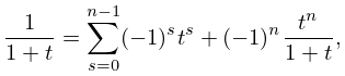
where $z=\rho e^{{i\theta}}$ , and $|\alpha|$ is bounded as $n\to\infty$ . From (2.11.5) and the identity

2.11.9 $\frac{1}{1+t}=\sum _{{s=0}}^{{n-1}}(-1)^{s}t^{s}+(-1)^{n}\frac{t^{n}}{1+t},$ $t\neq-1$ ,

Permalink:: http://dlmf.nist.gov/2.11.E9
Encodings:: TeX, pMML, png

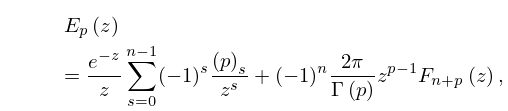
we have

2.11.10 $\mathop{E_{{p}}\/}\nolimits\!\left(z\right)=\frac{e^{{-z}}}{z}\sum _{{s=0}}^{{n-1}}(-1)^{s}\frac{\left(p\right)_{{s}}}{z^{s}}+(-1)^{n}\frac{2\pi}{\mathop{\Gamma\/}\nolimits\!\left(p\right)}z^{{p-1}}F_{{n+p}}(z),$

Symbols:: $\mathop{\Gamma\/}\nolimits\!\left(z\right)$ : gamma function, $\left(a\right)_{{n}}$ : Pochhammer’s symbol, $e$ : base of exponential function, $\mathop{E_{{p}}\/}\nolimits\!\left(z\right)$ : generalized exponential integral and $F_{{n+p}}(z)$ : function
Referenced by:: §2.11(iii), §2.11(iv)
Permalink:: http://dlmf.nist.gov/2.11.E10
Encodings:: TeX, pMML, png

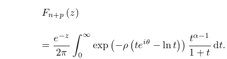
where

2.11.11 $F_{{n+p}}(z)=\frac{e^{{-z}}}{2\pi}\int _{{0}}^{{\infty}}\frac{e^{{-zt}}t^{{n+p-1}}}{1+t}dt=\frac{\mathop{\Gamma\/}\nolimits\!\left(n+p\right)}{2\pi}\frac{\mathop{E_{{n+p}}\/}\nolimits\!\left(z\right)}{z^{{n+p-1}}}.$

Symbols:: $\mathop{\Gamma\/}\nolimits\!\left(z\right)$ : gamma function, $dx$ : differential of $x$ , $e$ : base of exponential function, $\mathop{E_{{p}}\/}\nolimits\!\left(z\right)$ : generalized exponential integral, $\int$ : integral and $F_{{n+p}}(z)$ : function
Permalink:: http://dlmf.nist.gov/2.11.E11
Encodings:: TeX, pMML, png

With $n$ given by (2.11.8), we have

2.11.12 $F_{{n+p}}(z)=\frac{e^{{-z}}}{2\pi}\int _{{0}}^{{\infty}}\mathop{\exp\/}\nolimits\!\left(-\rho\left(te^{{i\theta}}-\mathop{\ln\/}\nolimits t\right)\right)\frac{t^{{\alpha-1}}}{1+t}dt.$

Symbols:: $dx$ : differential of $x$ , $\mathop{\exp\/}\nolimits z$ : exponential function, $e$ : base of exponential function, $\int$ : integral, $\mathop{\ln\/}\nolimits z$ : principal branch of logarithm function, $\rho$ : radius, $\theta$ : radius and $F_{{n+p}}(z)$ : function
Permalink:: http://dlmf.nist.gov/2.11.E12
Encodings:: TeX, pMML, png

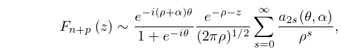
For large $\rho$ the integrand has a saddle point at $t=e^{{-i\theta}}$ . Following §2.4(iv), we rotate the integration path through an angle $-\theta$ , which is valid by analytic continuation when $-\pi<\theta<\pi$ . Then by application of Laplace’s method (§§2.4(iii) and 2.4(iv)), we have

2.11.13 $F_{{n+p}}(z)\sim\frac{e^{{-i(\rho+\alpha)\theta}}}{1+e^{{-i\theta}}}\frac{e^{{-\rho-z}}}{(2\pi\rho)^{{1/2}}}\sum _{{s=0}}^{{\infty}}\frac{a_{{2s}}(\theta,\alpha)}{\rho^{s}},$ $\rho\to\infty$ ,

Symbols:: $e$ : base of exponential function, $\sim$ : asymptotic equality, $\rho$ : radius, $\theta$ : radius, $F_{{n+p}}(z)$ : function and $a_{{2s}}(\theta,\alpha)$ : coefficients
Referenced by:: §2.11(iii), §2.11(iii)
Permalink:: http://dlmf.nist.gov/2.11.E13
Encodings:: TeX, pMML, png

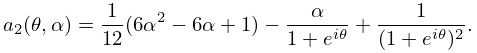
uniformly when $\theta\in[-\pi+\delta,\pi-\delta]$ ( $\delta>0$ ) and $|\alpha|$ is bounded. The coefficients are rational functions of $\alpha$ and $1+e^{{i\theta}}$ , for example, $a_{0}(\theta,\alpha)=1$ , and

2.11.14 $a_{2}(\theta,\alpha)=\frac{1}{12}(6\alpha^{2}-6\alpha+1)-\frac{\alpha}{1+e^{{i\theta}}}+\frac{1}{(1+e^{{i\theta}})^{2}}.$

Symbols:: $e$ : base of exponential function, $\theta$ : radius and $a_{{2s}}(\theta,\alpha)$ : coefficients
Referenced by:: §2.11(iii)
Permalink:: http://dlmf.nist.gov/2.11.E14
Encodings:: TeX, pMML, png

Owing to the factor $e^{{-\rho}}$ , that is, $e^{{-|z|}}$ in (2.11.13), $F_{{n+p}}(z)$ is uniformly exponentially small compared with $\mathop{E_{{p}}\/}\nolimits\!\left(z\right)$ . For this reason the expansion of $\mathop{E_{{p}}\/}\nolimits\!\left(z\right)$ in $|\mathop{\mathrm{ph}\/}\nolimits z|\leq\pi-\delta$ supplied by (2.11.8), (2.11.10), and (2.11.13) is said to be exponentially improved.

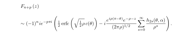
If we permit the use of nonelementary functions as approximants, then even more powerful re-expansions become available. One is uniformly valid for $-\pi+\delta\leq\mathop{\mathrm{ph}\/}\nolimits z\leq 3\pi-\delta$ with bounded $|\alpha|$ , and achieves uniform exponential improvement throughout $0\leq\mathop{\mathrm{ph}\/}\nolimits z\leq\pi$ :

2.11.15 $F_{{n+p}}(z)\sim(-1)^{n}ie^{{-p\pi i}}\left(\tfrac{1}{2}\mathop{\mathrm{erfc}\/}\nolimits\!\left(\sqrt{\tfrac{1}{2}\rho}\, c(\theta)\right)-i\frac{e^{{i\rho(\pi-\theta)}}e^{{-\rho-z}}}{(2\pi\rho)^{{1/2}}}\sum _{{s=0}}^{{\infty}}\frac{h_{{2s}}(\theta,\alpha)}{\rho^{s}}\right).$

Symbols:: $\mathop{\mathrm{erfc}\/}\nolimits z$ : complementary error function, $e$ : base of exponential function, $\sim$ : asymptotic equality, $\rho$ : radius, $\theta$ : radius, $F_{{n+p}}(z)$ : function, $c(\theta)$ and $h_{{2s}}(\theta,\alpha)$ : functions
Referenced by:: §2.11(iv), §2.11(iv), §2.11(v)
Permalink:: http://dlmf.nist.gov/2.11.E15
Encodings:: TeX, pMML, png

Here $\mathop{\mathrm{erfc}\/}\nolimits$ is the complementary error function (§7.2(i)), and

2.11.16 $c(\theta)=\sqrt{2(1+e^{{i\theta}}+i(\theta-\pi))},$

Symbols:: $e$ : base of exponential function, $\theta$ : radius and $c(\theta)$
Permalink:: http://dlmf.nist.gov/2.11.E16
Encodings:: TeX, pMML, png

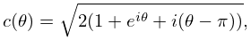
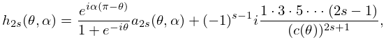
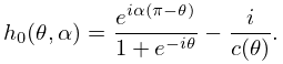
the branch being continuous with $c(\theta)\sim\pi-\theta$ as $\theta\to\pi$ . Also,

2.11.17 $h_{{2s}}(\theta,\alpha)=\frac{e^{{i\alpha(\pi-\theta)}}}{1+e^{{-i\theta}}}a_{{2s}}(\theta,\alpha)+(-1)^{{s-1}}i\frac{1\cdot 3\cdot 5\cdot\cdot\cdot(2s-1)}{(c(\theta))^{{2s+1}}},$

Symbols:: $e$ : base of exponential function, $\theta$ : radius, $a_{{2s}}(\theta,\alpha)$ : coefficients, $c(\theta)$ and $h_{{2s}}(\theta,\alpha)$ : functions
Permalink:: http://dlmf.nist.gov/2.11.E17
Encodings:: TeX, pMML, png

with $a_{{2s}}(\theta,\alpha)$ as in (2.11.13), (2.11.14). In particular,

2.11.18 $h_{0}(\theta,\alpha)=\frac{e^{{i\alpha(\pi-\theta)}}}{1+e^{{-i\theta}}}-\frac{i}{c(\theta)}.$

Symbols:: $e$ : base of exponential function, $\theta$ : radius, $c(\theta)$ and $h_{{2s}}(\theta,\alpha)$ : functions
Permalink:: http://dlmf.nist.gov/2.11.E18
Encodings:: TeX, pMML, png

For the sector $-3\pi+\delta\leq\mathop{\mathrm{ph}\/}\nolimits z\leq\pi-\delta$ the conjugate result applies.

Further details for this example are supplied in Olver (1991a, 1994b). See also Paris and Kaminski (2001, Chapter 6), and Dunster (1996b, 1997).

§2.11(iv) Stokes Phenomenon

Keywords:: Stokes line, Stokes phenomenon, asymptotic approximations and expansions
Referenced by:: §2.11(i), §2.11(ii), §2.11(vi), §6.12(i), §7.12(i), §7.20(i)
Permalink:: http://dlmf.nist.gov/2.11.iv

Two different asymptotic expansions in terms of elementary functions, (2.11.6) and (2.11.7), are available for the generalized exponential integral in the sector $\frac{1}{2}\pi<\mathop{\mathrm{ph}\/}\nolimits z<\frac{3}{2}\pi$ . That the change in their forms is discontinuous, even though the function being approximated is analytic, is an example of the Stokes phenomenon. Where should the change-over take place? Can it be accomplished smoothly?

Satisfactory answers to these questions were found by Berry (1989); see also the survey by Paris and Wood (1995). These answers are linked to the terms involving the complementary error function in the more powerful expansions typified by the combination of (2.11.10) and (2.11.15). Thus if $0\leq\theta\leq\pi-\delta$ ( $<\pi$ ), then $c(\theta)$ lies in the right half-plane. Hence from §7.12(i) $\mathop{\mathrm{erfc}\/}\nolimits\!\left(\sqrt{\frac{1}{2}\rho}\; c(\theta)\right)$ is of the same exponentially-small order of magnitude as the contribution from the other terms in (2.11.15) when $\rho$ is large. On the other hand, when $\pi+\delta\leq\theta\leq 3\pi-\delta$ , $c(\theta)$ is in the left half-plane and $\mathop{\mathrm{erfc}\/}\nolimits\!\left(\sqrt{\frac{1}{2}\rho}\; c(\theta)\right)$ differs from 2 by an exponentially-small quantity. In the transition through $\theta=\pi$ , $\mathop{\mathrm{erfc}\/}\nolimits\!\left(\sqrt{\frac{1}{2}\rho}\; c(\theta)\right)$ changes very rapidly, but smoothly, from one form to the other; compare the graph of its modulus in Figure 2.11.1 in the case $\rho=100$ .

Figure 2.11.1: Graph of $|\mathop{\mathrm{erfc}\/}\nolimits\!\left(\sqrt{50}\, c(\theta)\right)|$ .

Symbols:: $\mathop{\mathrm{erfc}\/}\nolimits z$ : complementary error function, $\theta$ : radius and $c(\theta)$
Referenced by:: §2.11(iv), §2.11(iv)
Permalink:: http://dlmf.nist.gov/2.11.F1
Encodings:: pdf, png

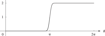
In particular, on the ray $\theta=\pi$ greatest accuracy is achieved by (a) taking the average of the expansions (2.11.6) and (2.11.7), followed by (b) taking account of the exponentially-small contributions arising from the terms involving $h_{{2s}}(\theta,\alpha)$ in (2.11.15).

Rays (or curves) on which one contribution in a compound asymptotic expansion achieves maximum dominance over another are called Stokes lines ( $\theta=\pi$ in the present example). As these lines are crossed exponentially-small contributions, such as that in (2.11.7), are “switched on” smoothly, in the manner of the graph in Figure 2.11.1.

For higher-order Stokes phenomena see Olde Daalhuis (2004b) and Howls et al. (2004).

§2.11(v) Exponentially-Improved Expansions (continued)

Keywords:: Borel transform theory, asymptotic approximations and expansions, asymptotic solutions of differential equations, hyperasymptotic expansions, resurgence, terminant function
Referenced by:: §10.46, §2.7(ii), §8.22(i)
Permalink:: http://dlmf.nist.gov/2.11.v

Expansions similar to (2.11.15) can be constructed for many other special functions. However, to enjoy the resurgence property (§2.7(ii)) we often seek instead expansions in terms of the $F$ -functions introduced in §2.11(iii), leaving the connection of the error-function type behavior as an implicit consequence of this property of the $F$ -functions. In this context the $F$ -functions are called terminants, a name introduced by Dingle (1973).

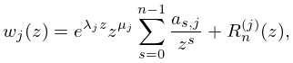
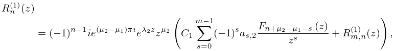
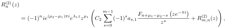
For illustration, we give re-expansions of the remainder terms in the expansions (2.7.8) arising in differential-equation theory. For notational convenience assume that the original differential equation (2.7.1) is normalized so that $\lambda _{2}-\lambda _{1}=1$ . (This means that, if necessary, $z$ is replaced by $z/(\lambda _{2}-\lambda _{1})$ .) From (2.7.12), (2.7.13) it is then seen that the optimum number of terms, $n$ , in (2.7.14) is approximately $|z|$ . We set

2.11.19 $w_{j}(z)=e^{{\lambda _{j}z}}z^{{\mu _{j}}}\sum _{{s=0}}^{{n-1}}\frac{a_{{s,j}}}{z^{s}}+R_{n}^{{(j)}}(z),$ $j=1,2$ ,

Symbols:: $e$ : base of exponential function, $a_{{s,j}}$ : coefficients, $R_{n}^{{(j)}}(z)$ : remainder, $\lambda _{j}$ : roots, $\mu _{j}$ : quantities and $w_{j}(z)$ : solutions
Permalink:: http://dlmf.nist.gov/2.11.E19
Encodings:: TeX, pMML, png

and expand

2.11.20 $R_{n}^{{(1)}}(z)=(-1)^{{n-1}}ie^{{(\mu _{2}-\mu _{1})\pi i}}e^{{\lambda _{2}z}}z^{{\mu _{2}}}\left(C_{1}\sum _{{s=0}}^{{m-1}}(-1)^{s}a_{{s,2}}\frac{F_{{n+\mu _{2}-\mu _{1}-s}}(z)}{z^{s}}+R_{{m,n}}^{{(1)}}(z)\right),$

Symbols:: $e$ : base of exponential function, $a_{{s,j}}$ : coefficients, $R_{n}^{{(j)}}(z)$ : remainder, $F_{{n+p}}(z)$ : function, $\lambda _{j}$ : roots, $\mu _{j}$ : quantities and $C_{1}$ , $C_{2}$ : Stokes multipliers
Referenced by:: §2.11(v)
Permalink:: http://dlmf.nist.gov/2.11.E20
Encodings:: TeX, pMML, png

2.11.21 $R_{n}^{{(2)}}(z)=(-1)^{n}ie^{{(\mu _{2}-\mu _{1})\pi i}}e^{{\lambda _{1}z}}z^{{\mu _{1}}}\left(C_{2}\sum _{{s=0}}^{{m-1}}(-1)^{s}a_{{s,1}}\frac{F_{{n+\mu _{1}-\mu _{2}-s}}(ze^{{-\pi i}})}{z^{s}}+R_{{m,n}}^{{(2)}}(z)\right),$

Symbols:: $e$ : base of exponential function, $a_{{s,j}}$ : coefficients, $R_{n}^{{(j)}}(z)$ : remainder, $F_{{n+p}}(z)$ : function, $\lambda _{j}$ : roots, $\mu _{j}$ : quantities and $C_{1}$ , $C_{2}$ : Stokes multipliers
Referenced by:: §2.11(v)
Permalink:: http://dlmf.nist.gov/2.11.E21
Encodings:: TeX, pMML, png

with $m=0,1,2,\dots$ , and $C_{1},C_{2}$ as in (2.7.17). Then as $z\to\infty$ , with $|n-|z||$ bounded and $m$ fixed,

2.11.22 $R_{{m,n}}^{{(1)}}(z)=\begin{cases}\mathop{O\/}\nolimits\!\left(e^{{-|z|-z}}z^{{-m}}\right),&|\mathop{\mathrm{ph}\/}\nolimits z|\leq\pi,\\ \mathop{O\/}\nolimits\!\left(z^{{-m}}\right),&\pi\leq|\mathop{\mathrm{ph}\/}\nolimits z|\leq\frac{5}{2}\pi-\delta,\end{cases}$

Symbols:: $\mathop{O\/}\nolimits\!\left(x\right)$ : order not exceeding, $e$ : base of exponential function, $\mathop{\mathrm{ph}\/}\nolimits$ : phase, $R_{n}^{{(j)}}(z)$ : remainder and $\delta$ : positive constant
Permalink:: http://dlmf.nist.gov/2.11.E22
Encodings:: TeX, pMML, png

2.11.23 $R_{{m,n}}^{{(2)}}(z)=\begin{cases}\mathop{O\/}\nolimits\!\left(e^{{-|z|+z}}z^{{-m}}\right),&0\leq\mathop{\mathrm{ph}\/}\nolimits z\leq 2\pi,\\ \mathop{O\/}\nolimits\!\left(z^{{-m}}\right),&-\frac{3}{2}\pi+\delta\leq\mathop{\mathrm{ph}\/}\nolimits z\leq 0\text{ and }2\pi\leq\mathop{\mathrm{ph}\/}\nolimits z\leq\frac{7}{2}\pi-\delta,\end{cases}$

Symbols:: $\mathop{O\/}\nolimits\!\left(x\right)$ : order not exceeding, $e$ : base of exponential function, $\mathop{\mathrm{ph}\/}\nolimits$ : phase, $R_{n}^{{(j)}}(z)$ : remainder and $\delta$ : positive constant
Permalink:: http://dlmf.nist.gov/2.11.E23
Encodings:: TeX, pMML, png

uniformly with respect to $\mathop{\mathrm{ph}\/}\nolimits z$ in each case.

The relevant Stokes lines are $\mathop{\mathrm{ph}\/}\nolimits z=\pm\pi$ for $w_{1}(z)$ , and $\mathop{\mathrm{ph}\/}\nolimits z=0,2\pi$ for $w_{2}(z)$ . In addition to achieving uniform exponential improvement, particularly in $|\mathop{\mathrm{ph}\/}\nolimits z|\leq\pi$ for $w_{1}(z)$ , and $0\leq\mathop{\mathrm{ph}\/}\nolimits z\leq 2\pi$ for $w_{2}(z)$ , the re-expansions (2.11.20), (2.11.21) are resurgent.

For further details see Olde Daalhuis and Olver (1994). For error bounds see Dunster (1996c). For other examples see Boyd (1990b), Paris (1992a, b), and Wong and Zhao (2002b).

Often the process of re-expansion can be repeated any number of times. In this way we arrive at hyperasymptotic expansions. For integrals, see Berry and Howls (1991), Howls (1992), and Paris and Kaminski (2001, Chapter 6). For second-order differential equations, see Olde Daalhuis and Olver (1995a), Olde Daalhuis (1995, 1996), and Murphy and Wood (1997).

For higher-order differential equations, see Olde Daalhuis (1998a, b). The first of these two references also provides an introduction to the powerful Borel transform theory. In this connection see also Byatt-Smith (2000).

For nonlinear differential equations see Olde Daalhuis (2005a, b).

For another approach see Paris (2001a, b).

§2.11(vi) Direct Numerical Transformations

Notes:: See Olver (1997b, pp. 540–543) and Weniger (1996). The computations in the example were carried out at NIST.
Keywords:: Euler’s transformation, Levin’s transformations, Whittaker functions, asymptotic approximations and expansions
Referenced by:: §3.9(vi)
Permalink:: http://dlmf.nist.gov/2.11.vi

The transformations in §3.9 for summing slowly convergent series can also be very effective when applied to divergent asymptotic series.

A simple example is provided by Euler’s transformation (§3.9(ii)) applied to the asymptotic expansion for the exponential integral (§6.12(i)):

2.11.24 $e^{x}\mathop{E_{1}\/}\nolimits\!\left(x\right)\sim\sum _{{s=0}}^{{\infty}}(-1)^{s}\frac{s!}{x^{{s+1}}},$ $x\to+\infty$ .

Symbols:: $e$ : base of exponential function, $\mathop{E_{1}\/}\nolimits\!\left(z\right)$ : exponential integral, $!$ : $n!$ : factorial and $\sim$ : asymptotic equality
Referenced by:: §2.11(vi)
Permalink:: http://dlmf.nist.gov/2.11.E24
Encodings:: TeX, pMML, png

Taking $x=5$ and rounding to 5D, we obtain

2.11.25 $e^{5}\mathop{E_{1}\/}\nolimits\!\left(5\right)=0.20000-0.04000+0.01600-0.00960+0.00768-0.00768+0.00922-0.01290+0.02064-0.03716+0.07432-\cdots.$

Symbols:: $e$ : base of exponential function and $\mathop{E_{1}\/}\nolimits\!\left(z\right)$ : exponential integral
Referenced by:: §2.11(vi)
Permalink:: http://dlmf.nist.gov/2.11.E25
Encodings:: TeX, pMML, png

The numerically smallest terms are the 5th and 6th. Truncation after 5 terms yields 0.17408, compared with the correct value

2.11.26 $e^{5}\mathop{E_{1}\/}\nolimits\!\left(5\right)=0.17042\dots.$

Symbols:: $e$ : base of exponential function and $\mathop{E_{1}\/}\nolimits\!\left(z\right)$ : exponential integral
Permalink:: http://dlmf.nist.gov/2.11.E26
Encodings:: TeX, pMML, png

We now compute the forward differences $\Delta^{j}$ , $j=0,1,2,\dots$ , of the moduli of the rounded values of the first 6 neglected terms:

2.11.27

$\Delta^{0}=0.00768$ ,

$\Delta^{1}=0.00154$ ,

$\Delta^{2}=0.00214$ ,

$\Delta^{3}=0.00192$ ,

$\Delta^{4}=0.00280$ ,

$\Delta^{5}=0.00434$ .

Symbols:: $\Delta^{j}$ : $j$ th forward difference
Permalink:: http://dlmf.nist.gov/2.11.E27
Encodings:: TeX, TeX, TeX, TeX, TeX, TeX, pMML, pMML, pMML, pMML, pMML, pMML, png, png, png, png, png, png

Multiplying these differences by $(-1)^{j}2^{{-j-1}}$ and summing, we obtain

2.11.28 $0.00384-0.00038+0.00027-0.00012+0.00009-0.00007=0.00363.$

Permalink:: http://dlmf.nist.gov/2.11.E28
Encodings:: TeX, pMML, png

Subtraction of this result from the sum of the first 5 terms in (2.11.25) yields 0.17045, which is much closer to the true value.

The process just used is equivalent to re-expanding the remainder term of the original asymptotic series (2.11.24) in powers of $1/(x+5)$ and truncating the new series optimally. Further improvements in accuracy can be realized by making a second application of the Euler transformation; see Olver (1997b, pp. 540–543).

Similar improvements are achievable by Aitken’s $\Delta^{2}$ -process, Wynn’s $\epsilon$ -algorithm, and other acceleration transformations. For a comprehensive survey see Weniger (1989).

The following example, based on Weniger (1996), illustrates their power.

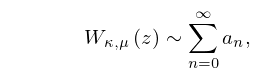
For large $|z|$ , with $|\mathop{\mathrm{ph}\/}\nolimits z|\leq\frac{3}{2}\pi-\delta$ ( $<\frac{3}{2}\pi$ ), the Whittaker function of the second kind has the asymptotic expansion (§13.19)

2.11.29 $\mathop{W_{{\kappa,\mu}}\/}\nolimits\!\left(z\right)\sim\sum _{{n=0}}^{{\infty}}a_{n},$

Symbols:: $\mathop{W_{{\kappa,\mu}}\/}\nolimits\!\left(z\right)$ : Whittaker confluent hypergeometric function, $\sim$ : asymptotic equality and $a_{n}$ : coefficients
Permalink:: http://dlmf.nist.gov/2.11.E29
Encodings:: TeX, pMML, png

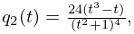
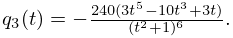
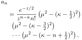
in which

2.11.30 $a_{n}=\frac{e^{{-z/2}}}{z^{{n-\kappa}}n!}\left(\mu^{2}-(\kappa-\tfrac{1}{2})^{2}\right)\*\left(\mu^{2}-(\kappa-\tfrac{3}{2})^{2}\right)\*\cdot\cdot\cdot\left(\mu^{2}-(\kappa-n+\tfrac{1}{2})^{2}\right).$

Symbols:: $e$ : base of exponential function, $!$ : $n!$ : factorial and $a_{n}$ : coefficients
Permalink:: http://dlmf.nist.gov/2.11.E30
Encodings:: TeX, pMML, png

With $z=1.0$ , $\kappa=2.3$ , $\mu=0.5$ , the values of $a_{n}$ to 8D are supplied in the second column of Table 2.11.1.

Table 2.11.1: Whittaker functions with Levin’s transformation.

$n$	$a_{{n}}$	$s_{{n}}$	$d_{{n}}$
0	0.60653 066	0.60653 066	0.60653 066
1	−1.81352 667	−1.20699 601	−0.91106 488
2	0.35363 770	−0.85335 831	−0.82413 405
3	0.02475 464	−0.82860 367	−0.83323 429
4	−0.00736 451	−0.83596 818	−0.83303 750
5	0.00676 062	−0.82920 756	−0.83298 901
6	−0.01125 643	−0.84046 399	−0.83299 429
7	0.02796 418	−0.81249 981	−0.83299 530
8	−0.09364 504	−0.90614 485	−0.83299 504
9	0.39736 710	−0.50877 775	−0.83299 501
10	−2.05001 686	−2.55879 461	−0.83299 503

Symbols:: $a_{n}$ : coefficients and $d_{n}$ : coeffient
Referenced by:: §2.11(vi), §2.11(vi)
Permalink:: http://dlmf.nist.gov/2.11.T1

The next column lists the partial sums $s_{n}=a_{0}+a_{1}+\dots+a_{n}$ . Optimum truncation occurs just prior to the numerically smallest term, that is, at $s_{4}$ . Comparison with the true value

2.11.31 $\mathop{W_{{2.3,0.5}}\/}\nolimits\!\left(1.0\right)=-0.83299\; 50268\; 27526\;\cdots$

Symbols:: $\mathop{W_{{\kappa,\mu}}\/}\nolimits\!\left(z\right)$ : Whittaker confluent hypergeometric function
Referenced by:: §2.11(vi)
Permalink:: http://dlmf.nist.gov/2.11.E31
Encodings:: TeX, pMML, png

shows that this direct estimate is correct to almost 3D.

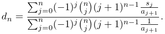
The fourth column of Table 2.11.1 gives the results of applying the following variant of Levin’s transformation:

2.11.32 $d_{n}=\frac{\sum _{{j=0}}^{{n}}(-1)^{j}\binom{n}{j}(j+1)^{{n-1}}\frac{s_{j}}{a_{{j+1}}}}{\sum _{{j=0}}^{{n}}(-1)^{j}\binom{n}{j}(j+1)^{{n-1}}\frac{1}{a_{{j+1}}}}.$

Symbols:: $\binom{m}{n}$ : binomial coefficient, $a_{n}$ : coefficients and $d_{n}$ : coeffient
Permalink:: http://dlmf.nist.gov/2.11.E32
Encodings:: TeX, pMML, png

By $n=10$ we already have 8 correct decimals. Furthermore, on proceeding to higher values of $n$ with higher precision, much more accuracy is achievable. For example, using double precision $d_{{20}}$ is found to agree with (2.11.31) to 13D.

However, direct numerical transformations need to be used with care. Their extrapolation is based on assumed forms of remainder terms that may not always be appropriate for asymptotic expansions. For example, extrapolated values may converge to an accurate value on one side of a Stokes line (§2.11(iv)), and converge to a quite inaccurate value on the other.