How to Buy Cenforce 100 - www.RxLara.com - Cenforce 200 price. For ED over the counter Visit - RXLARA.COM

SearchAdvancedHelp

(0.005 seconds)

11—20 of 868 matching pages

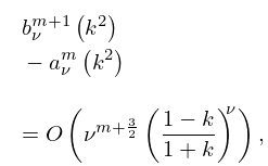
11: 29.7 Asymptotic Expansions

… ►As $\nu \to \mathrm{\infty }$, … ►

29.7.5 $$b_{\nu }^{m+1}\left(k^2\right)-a_{\nu }^m\left(k^2\right)=O\left({\nu }^{m+\frac{3}{2}}{\left(\frac{1-k}{1+k}\right)}^{\nu }\right),$$ $\nu \to \mathrm{\infty }$.

ⓘ

Symbols:

$O\left(x\right)$: order not exceeding, $a_{\nu }^n\left(k^2\right)$: eigenvalues of Lamé’s equation, $b_{\nu }^n\left(k^2\right)$: eigenvalues of Lamé’s equation, $m$: nonnegative integer, $k$: real parameter and $\nu$: real parameter

Referenced by:

§29.7(i)

Permalink:

http://dlmf.nist.gov/29.7.E5

Encodings:

pMML, png, TeX

See also:

Annotations for §29.7(i), §29.7 and Ch.29

… ►Müller (1966a, b) found three formal asymptotic expansions for a fundamental system of solutions of (29.2.1) (and (29.11.1)) as $\nu \to \mathrm{\infty }$, one in terms of Jacobian elliptic functions and two in terms of Hermite polynomials. In Müller (1966c) it is shown how these expansions lead to asymptotic expansions for the Lamé functions ${\mathrm{𝐸𝑐}}_{\nu }^m(z,k^2)$ and ${\mathrm{𝐸𝑠}}_{\nu }^m(z,k^2)$. Weinstein and Keller (1985) give asymptotics for solutions of Hill’s equation (§28.29(i)) that are applicable to the Lamé equation.

12: Bibliography G

… ►

Orthogonality of certain functions with respect to complex valued weights. Canad. J. Math. 33 (5), pp. 1261–1270.

ⓘ

External Links:

ISSN 0008-414X, MathReview (Mourad E. H. Ismail), ZentralBlatt

Referenced by:

§18.33(v).

Encodings:

BibTeX

… ►

Some elementary inequalities relating to the gamma and incomplete gamma function. J. Math. Phys. 38 (1), pp. 77–81.

ⓘ

External Links:

MathReview (H. O. Pollak), ZentralBlatt

Referenced by:

§5.6(i), §6.8, §7.8, §8.10.

Encodings:

BibTeX

… ►

How and how not to check Gaussian quadrature formulae. BIT 23 (2), pp. 209–216.

ⓘ

External Links:

ISSN 0006-3835, Document, MathReview (G. A. Evans), ZentralBlatt

Referenced by:

§18.40(ii), §3.5(v), §9.17(iii).

Encodings:

BibTeX

►

Questions of Numerical Condition Related to Polynomials. In Studies in Numerical Analysis, G. H. Golub (Ed.), pp. 140–177.

ⓘ

External Links:

MathReview Entry, ZentralBlatt

Referenced by:

§3.8(vi).

Encodings:

BibTeX

… ►

Linear Differential Equations and Group Theory from Riemann to Poincaré. 2nd edition, Birkhäuser Boston Inc., Boston, MA.

ⓘ

External Links:

ISBN 0-8176-3837-7, MathReview, ZentralBlatt

Referenced by:

§15.17(v).

Encodings:

BibTeX

…

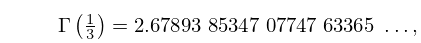
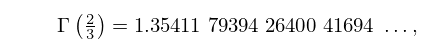
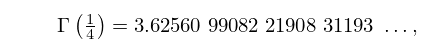
13: 5.4 Special Values and Extrema

… ►

5.4.7 $$\mathrm{\Gamma }\left(\frac{1}{3}\right)=\mathrm{2.67893\hspace{0.33em}85347\hspace{0.33em}07747\hspace{0.33em}63365}\mathrm{\dots },$$

ⓘ

Symbols:

$\mathrm{\Gamma }\left(z\right)$: gamma function

A&S Ref:

6.1.11 (where the value is computed to 10D.)

Notes:

For more digits see OEIS Sequence A073005; see also Sloane (2003).

Permalink:

http://dlmf.nist.gov/5.4.E7

Encodings:

pMML, png, TeX

See also:

Annotations for §5.4(i), §5.4 and Ch.5

►

5.4.8 $$\mathrm{\Gamma }\left(\frac{2}{3}\right)=\mathrm{1.35411\hspace{0.33em}79394\hspace{0.33em}26400\hspace{0.33em}41694}\mathrm{\dots },$$

ⓘ

Symbols:

$\mathrm{\Gamma }\left(z\right)$: gamma function

A&S Ref:

6.1.13 (where the value is computed to 10D.)

Notes:

For more digits see OEIS Sequence A073006; see also Sloane (2003).

Permalink:

http://dlmf.nist.gov/5.4.E8

Encodings:

pMML, png, TeX

See also:

Annotations for §5.4(i), §5.4 and Ch.5

►

5.4.9 $$\mathrm{\Gamma }\left(\frac{1}{4}\right)=\mathrm{3.62560\hspace{0.33em}99082\hspace{0.33em}21908\hspace{0.33em}31193}\mathrm{\dots },$$

ⓘ

Symbols:

$\mathrm{\Gamma }\left(z\right)$: gamma function

A&S Ref:

6.1.10 (where the value is computed to 10D.)

Notes:

For more digits see OEIS Sequence A068466; see also Sloane (2003).

Permalink:

http://dlmf.nist.gov/5.4.E9

Encodings:

pMML, png, TeX

See also:

Annotations for §5.4(i), §5.4 and Ch.5

►

5.4.10 $$\mathrm{\Gamma }\left(\frac{3}{4}\right)=\mathrm{1.22541\hspace{0.33em}67024\hspace{0.33em}65177\hspace{0.33em}64512}\mathrm{\dots }.$$

ⓘ

Symbols:

$\mathrm{\Gamma }\left(z\right)$: gamma function

A&S Ref:

6.1.14 (where the value is computed to 10D.)

Notes:

For more digits see OEIS Sequence A068465; see also Sloane (2003).

Permalink:

http://dlmf.nist.gov/5.4.E10

Encodings:

pMML, png, TeX

See also:

Annotations for §5.4(i), §5.4 and Ch.5

… ►As $n\to \mathrm{\infty }$, …

14: 10.74 Methods of Computation

… ►In other circumstances the power series are prone to slow convergence and heavy numerical cancellation. … ►Temme (1997) shows how to overcome this difficulty by use of the Maclaurin expansions for these coefficients or by use of auxiliary functions. … ►Similar observations apply to the computation of modified Bessel functions, spherical Bessel functions, and Kelvin functions. … ►Similar considerations apply to the spherical Bessel functions and Kelvin functions. … ►Newton’s rule (§3.8(i)) or Halley’s rule (§3.8(v)) can be used to compute to arbitrarily high accuracy the real or complex zeros of all the functions treated in this chapter. …

15: 22.20 Methods of Computation

… ►To compute $\mathrm{sn}$, $\mathrm{cn}$, $\mathrm{dn}$ to 10D when $x=0.8$, $k=0.65$. ►Four iterations of (22.20.1) lead to $c_4=\mathrm{6.5\times 10⁻¹²}$. … ►By application of the transformations given in §§22.7(i) and 22.7(ii), $k$ or $k^{\prime }$ can always be made sufficently small to enable the approximations given in §22.10(ii) to be applied. The rate of convergence is similar to that for the arithmetic-geometric mean. … ►Alternatively, Sala (1989) shows how to apply the arithmetic-geometric mean to compute $\mathrm{am}(x,k)$. …

16: 3.6 Linear Difference Equations

… ►In practice, however, problems of severe instability often arise and in §§3.6(ii)–3.6(vii) we show how these difficulties may be overcome. … ►It therefore remains to apply a normalizing factor $\mathrm{\Lambda }$. … ►(This part of the process is equivalent to forward elimination.) … ►Similar considerations apply to the first-order equation …Thus in the inhomogeneous case it may sometimes be necessary to recur backwards to achieve stability. …

17: Errata

… ►

The paragraph immediately below (9.8.23) was updated to include new information from Nemes (2021) pertaining to (9.8.22) and (9.8.23).

… ►

In the paragraph immediately below (25.10.4), it was originally stated that “more than one-third of all zeros in the critical strip lie on the critical line.” which referred to Levinson (1974). This sentence has been updated with “one-third” being replaced with “41%” now referring to Bui et al. (2011) (suggested by Gergő Nemes on 2021-08-23).

… ►

In Equation (1.13.4), the determinant form of the two-argument Wronskian

1.13.4

was added as an equality. In ¶Wronskian (in §1.13(i)), immediately below Equation (1.13.4), a sentence was added indicating that in general the $n$-argument Wronskian is given by $𝒲\left\{w_1(z),\mathrm{\dots },w_n(z)\right\}=det\left[w_k^{(j-1)}(z)\right]$, where $1\le j,k\le n$. Immediately below Equation (1.13.4), a sentence was added giving the definition of the $n$-argument Wronskian. It is explained just above (1.13.5) that this equation is often referred to as Abel’s identity. Immediately below Equation (1.13.5), a sentence was added explaining how it generalizes for $n$th-order differential equations. A reference to Ince (1926, §5.2) was added.

… ►

Additional keywords are being added to formulas (an ongoing project); these are visible in the associated ‘info boxes’ linked to the icons to the right of each formula, and provide better search capabilities.

… ►

A number of additions and changes have been made to the metadata to reflect new and changed references as well as to how some equations have been derived.

…

18: 3.2 Linear Algebra

… ►To solve the system … ►During this reduction process we store the multipliers ${\mathrm{\ell }}_{jk}$ that are used in each column to eliminate other elements in that column. … ►The sensitivity of the solution vector $𝐱$ in (3.2.1) to small perturbations in the matrix $𝐀$ and the vector $𝐛$ is measured by the condition number … ►where $𝐱$ and $𝐲$ are the normalized right and left eigenvectors of $𝐀$ corresponding to the eigenvalue $\lambda$. … ►Lanczos’ method is related to Gauss quadrature considered in §3.5(v). …

19: 25.10 Zeros

… ►Calculations relating to the zeros on the critical line make use of the real-valued function …is chosen to make $Z(t)$ real, and $\mathrm{ph}\mathrm{\Gamma }\left(\frac{1}{4}+\frac{1}{2}\mathrm{i}t\right)$ assumes its principal value. … ►Sign changes of $Z(t)$ are determined by multiplying (25.9.3) by $\exp \left(\mathrm{i}\vartheta (t)\right)$ to obtain the Riemann–Siegel formula: …where $R(t)=O\left(t^{-1/4}\right)$ as $t\to \mathrm{\infty }$. … ►More than 41% of all the zeros in the critical strip lie on the critical line (Bui et al. (2011)). …

20: Bibliography B

… ►

An Introduction to Linear Difference Equations. Dover Publications Inc., New York.

ⓘ

Notes:

Unaltered republication of the original 1927 Harvard University edition.

External Links:

MathReview, ZentralBlatt

Referenced by:

§8.1, Notations P, Notations Q.

Encodings:

BibTeX

… ►

The fifty-two icosahedral solutions to Painlevé VI. J. Reine Angew. Math. 596, pp. 183–214.

ⓘ

External Links:

ISSN 0075-4102, Document, MathReview (Andrei A. Kapaev), ZentralBlatt

Referenced by:

§32.9(iii).

Encodings:

BibTeX

… ►

Irregular primes to one million. Math. Comp. 59 (200), pp. 717–722.

ⓘ

External Links:

ISSN 0025-5718, FullText, MathReview (Duncan A. Buell), ZentralBlatt

Referenced by:

2nd item.

Encodings:

BibTeX

… ►

More than 41% of the zeros of the zeta function are on the critical line. Acta Arith. 150 (1), pp. 35–64.

ⓘ

External Links:

ISSN 0065-1036, Document, Link, MathReview (Timothy S. Trudgian), ZentralBlatt

Referenced by:

§25.10(ii), §25.10(ii), Erratum (V1.1.4) for Subsection 25.10(ii).

Encodings:

BibTeX

… ►

A Guide to Mathematical Tables: Supplement No. 1. Pergamon Press, New York.

ⓘ

Notes:

Supplement to “A Guide to Mathematical Tables” by A. V. Lebedev and R. M. Fedorova.

External Links:

MathReview

Referenced by:

A. V. Lebedev and R. M. Fedorova (1960).

Encodings:

BibTeX

…