§22.20 Methods of Computation
Contents
- §22.20(i) Via Theta Functions
- §22.20(ii) Arithmetic-Geometric Mean
- §22.20(iii) Landen Transformations
- §22.20(iv) Lattice Calculations
- §22.20(v) Inverse Functions
- §22.20(vi) Related Functions
- §22.20(vii) Further References
§22.20(i) Via Theta Functions
§22.20(ii) Arithmetic-Geometric Mean
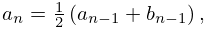
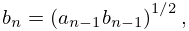
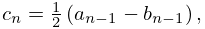
Given real or complex numbers , with not real and negative, define
| 22.20.1 | ||||
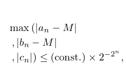
for , where the square root is chosen so that , where and are chosen so that their difference is numerically less than . Then as sequences , converge to a common limit , the arithmetic-geometric mean of . And since
| 22.20.2 | |||
convergence is very rapid.
For real and , use (22.20.1) with , , , and continue until is zero to the required accuracy. Next, compute , where
| 22.20.3 | |||
| 22.20.4 | |||
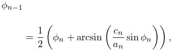
and the inverse sine has its principal value (§4.23(ii)). Then
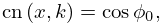
| 22.20.5 | ||||
and the subsidiary functions can be found using (22.2.10). This formula for becomes unstable near . If only the value of at is required then the exact value is in the table 22.5.1. If both and are real then is strictly positive and which follows from (22.6.1). If either or is complex then (22.2.6) gives the definition of as a quotient of theta functions.
See also Wachspress (2000).
Example
To compute , , to 10D when , .
§22.20(iii) Landen Transformations
By application of the transformations given in §§22.7(i) and 22.7(ii), or can always be made sufficently small to enable the approximations given in §22.10(ii) to be applied. The rate of convergence is similar to that for the arithmetic-geometric mean.
Example
To compute to 6D for , , .
§22.20(iv) Lattice Calculations
If either or is given, then we use , , , and , obtaining the values of the theta functions as in §20.14.
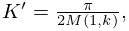
If are given with and , then can be found from
| 22.20.6 | ||||
using the arithmetic-geometric mean.
Example 1
Example 2
If , then four iterations of (22.20.1) give .
§22.20(v) Inverse Functions
See Wachspress (2000).
