§1.13 Differential Equations
Contents
- §1.13(i) Existence of Solutions
- §1.13(ii) Equations with a Parameter
- §1.13(iii) Inhomogeneous Equations
- §1.13(iv) Change of Variables
- §1.13(v) Products of Solutions
- §1.13(vi) Singularities
- §1.13(vii) Closed-Form Solutions
- §1.13(viii) Eigenvalues and Eigenfunctions: Sturm-Liouville and Liouville forms
§1.13(i) Existence of Solutions
A domain in the complex plane is simply-connected if it has no “holes”; more precisely, if its complement in the extended plane is connected.
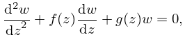
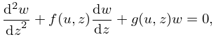
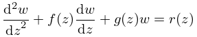
The equation
| 1.13.1 | |||
where , a simply-connected domain, and , are analytic in , has an infinite number of analytic solutions in . A solution becomes unique, for example, when and are prescribed at a point in .
Fundamental Pair
Two solutions and are called a fundamental pair if any other solution is expressible as
| 1.13.2 | |||
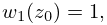
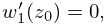
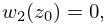
where and are constants. A fundamental pair can be obtained, for example, by taking any and requiring that
| 1.13.3 | ||||
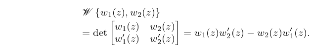
Wronskian
The Wronskian of and is defined by
| 1.13.4 | |||
(More generally , where .) Then the following relation is known as Abel’s identity
| 1.13.5 | |||
where is independent of and is defined in (1.13.1). (More generally in (1.13.5) for th-order differential equations, is the coefficient multiplying the th-order derivative of the solution divided by the coefficient multiplying the th-order derivative of the solution, see Ince (1926, §5.2).) If , then the Wronskian is constant.
The following three statements are equivalent: and comprise a fundamental pair in ; does not vanish in ; and are linearly independent, that is, the only constants and such that
| 1.13.6 | |||
| , | |||
are .
§1.13(ii) Equations with a Parameter
Assume that in the equation
| 1.13.7 | |||
and belong to domains and respectively, the coefficients and are continuous functions of both variables, and for each fixed (fixed ) the two functions are analytic in (in ). Suppose also that at (a fixed) , and are analytic functions of . Then at each , , and are analytic functions of .
§1.13(iii) Inhomogeneous Equations
The inhomogeneous (or nonhomogeneous) equation
| 1.13.8 | |||
with , , and analytic in has infinitely many analytic solutions in . If is any one solution, and , are a fundamental pair of solutions of the corresponding homogeneous equation (1.13.1), then every solution of (1.13.8) can be expressed as
| 1.13.9 | |||
where and are constants.
Variation of Parameters
§1.13(iv) Change of Variables
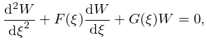
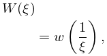
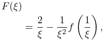
Transformation of the Point at Infinity
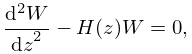
Elimination of First Derivative by Change of Dependent Variable
Elimination of First Derivative by Change of Independent Variable
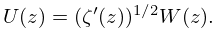
Liouville Transformation
Let satisfy (1.13.14), be any thrice-differentiable function of , and
| 1.13.18 | |||
Then
| 1.13.19 | |||
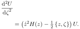
Here dots denote differentiations with respect to , and is the Schwarzian derivative:
| 1.13.20 | |||
Cayley’s Identity
For arbitrary and ,
| 1.13.21 | ||||
| 1.13.22 | ||||
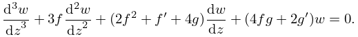
§1.13(v) Products of Solutions
The product of any two solutions of (1.13.1) satisfies
| 1.13.23 | |||
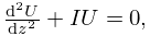
If and are respectively solutions of
| 1.13.24 | ||||
then is a solution of
| 1.13.25 | |||
For extensions of these results to linear homogeneous differential equations of arbitrary order see Spigler (1984).
§1.13(vi) Singularities
§1.13(vii) Closed-Form Solutions
For an extensive collection of solutions of differential equations of the first, second, and higher orders see Kamke (1977).
§1.13(viii) Eigenvalues and Eigenfunctions: Sturm-Liouville and Liouville forms
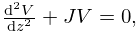
A standard form for second order ordinary differential equations with , and with a real parameter , and real valued functions and , with and positive, is
| 1.13.26 | |||
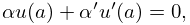
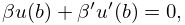
This is the Sturm-Liouville form of a second order differential equation, where ′ denotes . Assuming that satisfies un-mixed boundary conditions of the form
| 1.13.27 | ||||
| , not both zero, | ||||
| , not both zero, | ||||
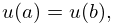
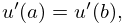
or periodic boundary conditions
| 1.13.28 | ||||
on a finite interval , this is then a regular Sturm-Liouville system.
Eigenvalues and Eigenfunctions
Transformation to Liouville normal Form
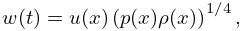
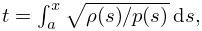
Equation (1.13.26) with may be transformed to the Liouville normal form
| 1.13.29 | |||
where now denotes , via the transformation
| 1.13.30 | ||||
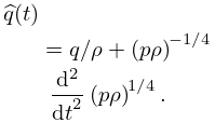
and where
| 1.13.31 | |||
As the interval is mapped, one-to-one, onto by the above definition of , the integrand being positive, the inverse of this same transformation allows to be calculated from in (1.13.31), and .
For a regular Sturm-Liouville system, equations (1.13.26) and (1.13.29) have: (i) identical eigenvalues, ; (ii) the corresponding (real) eigenfunctions, and , have the same number of zeros, also called nodes, for as for ; (iii) the eigenfunctions also satisfy the same type of boundary conditions, un-mixed or periodic, for both forms at the corresponding boundary points. See Birkhoff and Rota (1989, §§10.9, 10.10), Everitt (1982, §4.3), Olver (1997b, Ch. 6).
