28 Mathieu Functions and Hill’s Equation Hill’s Equation 28.28 Integrals, Integral Representations, and Integral Equations 28.30 Expansions in Series of Eigenfunctions

§28.29 Definitions and Basic Properties

Referenced by:: Ch.28
Permalink:: http://dlmf.nist.gov/28.29

§28.29(i) Hill’s Equation
§28.29(ii) Floquet’s Theorem and the Characteristic Exponent
§28.29(iii) Discriminant and Eigenvalues in the Real Case

§28.29(i) Hill’s Equation

Notes:: See Magnus and Winkler (1966, p. 8), Arscott (1964b, §7.1), and McLachlan (1947, §6.10).
Keywords:: Hill’s equation
Referenced by:: §29.7(ii)
Permalink:: http://dlmf.nist.gov/28.29.i

A generalization of Mathieu’s equation (28.2.1) is Hill’s equation

28.29.1 $w^{{\prime\prime}}(z)+\left(\lambda+Q(z)\right)w=0,$

Symbols:: : complex variable, : Mathieu’s equation solution, $\lambda$ : parameter and : function
Referenced by:: §28.29(ii), §28.29(ii), §28.29(ii), §28.29(iii), §28.29(iii), §28.29(iii)
Permalink:: http://dlmf.nist.gov/28.29.E1
Encodings:: TeX, pMML, png

with

28.29.2 $Q(z+\pi)=Q(z),$

Symbols:: : complex variable and : function
Permalink:: http://dlmf.nist.gov/28.29.E2
Encodings:: TeX, pMML, png

and

28.29.3 $\int_{0}^{\pi}Q(z)dz=0.$

Symbols:: : differential of , $\int$ : integral, : complex variable and : function
Permalink:: http://dlmf.nist.gov/28.29.E3
Encodings:: TeX, pMML, png

is either a continuous and real-valued function for $z\in\Real$ or an analytic function of in a doubly-infinite open strip that contains the real axis. $\pi$ is the minimum period of .

§28.29(ii) Floquet’s Theorem and the Characteristic Exponent

Notes:: See Magnus and Winkler (1966, §§1.2 and 1.3).
Keywords:: Floquet solutions, Floquet’s theorem, Hill’s equation, characteristic equation, pseudoperiodic solutions
Permalink:: http://dlmf.nist.gov/28.29.ii

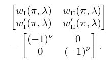
The basic solutions $w_{{\mbox{\tiny I}}}(z,\lambda)$ , $w_{{\mbox{\tiny II}}}(z,\lambda)$ are defined in the same way as in §28.2(ii) (compare (28.2.5), (28.2.6)). Then

28.29.4 $w_{{\mbox{\tiny I}}}(z+\pi,\lambda)=w_{{\mbox{\tiny I}}}(\pi,\lambda)w_{{\mbox% {\tiny I}}}(z,\lambda)+w^{{\prime}}_{{\mbox{\tiny I}}}(\pi,\lambda)w_{{\mbox{% \tiny II}}}(z,\lambda),$

Symbols:: : complex variable, : Mathieu’s equation solution, $w_{{\mbox{\tiny I}}}(z;a,q)$ : fundamental solution, $w_{{\mbox{\tiny II}}}(z;a,q)$ : fundamental solution and $\lambda$ : parameter
Permalink:: http://dlmf.nist.gov/28.29.E4
Encodings:: TeX, pMML, png

28.29.5 $w_{{\mbox{\tiny II}}}(z+\pi,\lambda)=w_{{\mbox{\tiny II}}}(\pi,\lambda)w_{{% \mbox{\tiny I}}}(z,\lambda)+w^{{\prime}}_{{\mbox{\tiny II}}}(\pi,\lambda)w_{{% \mbox{\tiny II}}}(z,\lambda).$

Symbols:: : complex variable, : Mathieu’s equation solution, $w_{{\mbox{\tiny I}}}(z;a,q)$ : fundamental solution, $w_{{\mbox{\tiny II}}}(z;a,q)$ : fundamental solution and $\lambda$ : parameter
Permalink:: http://dlmf.nist.gov/28.29.E5
Encodings:: TeX, pMML, png

Let $\nu$ be a real or complex constant satisfying (without loss of generality)

28.29.6 $-1<\realpart{\nu}\leq 1$

Symbols:: $\realpart{}$ : real part and $\nu$ : complex parameter
Referenced by:: §28.29(ii)
Permalink:: http://dlmf.nist.gov/28.29.E6
Encodings:: TeX, pMML, png

throughout this section. Then (28.29.1) has a nontrivial solution with the pseudoperiodic property

28.29.7 $w(z+\pi)=e^{{\pi i\nu}}w(z),$

Symbols:: : base of exponential function, : complex variable, $\nu$ : complex parameter and : Mathieu’s equation solution
Referenced by:: §28.29(ii)
Permalink:: http://dlmf.nist.gov/28.29.E7
Encodings:: TeX, pMML, png

iff $e^{{\pi i\nu}}$ is an eigenvalue of the matrix

28.29.8 $\begin{bmatrix}w_{{\mbox{\tiny I}}}(\pi,\lambda)&w_{{\mbox{\tiny II}}}(\pi,% \lambda)\\ w^{{\prime}}_{{\mbox{\tiny I}}}(\pi,\lambda)&w^{{\prime}}_{{\mbox{\tiny II}}}(% \pi,\lambda)\end{bmatrix}.$

Symbols:: : Mathieu’s equation solution, $w_{{\mbox{\tiny I}}}(z;a,q)$ : fundamental solution, $w_{{\mbox{\tiny II}}}(z;a,q)$ : fundamental solution and $\lambda$ : parameter
Permalink:: http://dlmf.nist.gov/28.29.E8
Encodings:: TeX, pMML, png

Equivalently,

28.29.9 $2\mathop{\cos\/}\nolimits\!\left(\pi\nu\right)=w_{{\mbox{\tiny I}}}(\pi,% \lambda)+w_{{\mbox{\tiny II}}}^{{\prime}}(\pi,\lambda).$

Symbols:: $\mathop{\cos\/}\nolimits z$ : cosine function, $\nu$ : complex parameter, $w_{{\mbox{\tiny I}}}(z;a,q)$ : fundamental solution, $w_{{\mbox{\tiny II}}}(z;a,q)$ : fundamental solution and $\lambda$ : parameter
Referenced by:: §28.29(ii), §28.29(ii), §28.29(ii)
Permalink:: http://dlmf.nist.gov/28.29.E9
Encodings:: TeX, pMML, png

This is the characteristic equation of (28.29.1), and $\mathop{\cos\/}\nolimits\!\left(\pi\nu\right)$ is an entire function of $\lambda$ . Given $\lambda$ together with the condition (28.29.6), the solutions $\pm\nu$ of (28.29.9) are the characteristic exponents of (28.29.1). A solution satisfying (28.29.7) is called a Floquet solution with respect to $\nu$ (or Floquet solution). It has the form

28.29.10 $F_{{\nu}}(z)=e^{{i\nu z}}P_{{\nu}}(z),$

Symbols:: : base of exponential function, : complex variable, $\nu$ : complex parameter and $F_{{\nu}}(z)$ : Floquet solution
Permalink:: http://dlmf.nist.gov/28.29.E10
Encodings:: TeX, pMML, png

where the function $P_{{\nu}}(z)$ is $\pi$ -periodic.

If $\nu$ $(\neq 0,1)$ is a solution of (28.29.9), then $F_{\nu}(z)$ , $F_{{-\nu}}(z)$ comprise a fundamental pair of solutions of Hill’s equation.

If $\nu=0$ or 1, then (28.29.1) has a nontrivial solution which is periodic with period $\pi$ (when $\nu=0$ ) or $2\pi$ (when $\nu=1$ ). Let be a solution linearly independent of . Then

28.29.11 $w(z+\pi)=(-1)^{{\nu}}w(z)+cP(z),$

Symbols:: : complex variable, $\nu$ : complex parameter, : Mathieu’s equation solution and : constant
Permalink:: http://dlmf.nist.gov/28.29.E11
Encodings:: TeX, pMML, png

where is a constant. The case is equivalent to

28.29.12 $\begin{bmatrix}w_{{\mbox{\tiny I}}}(\pi,\lambda)&w_{{\mbox{\tiny II}}}(\pi,% \lambda)\\ w^{{\prime}}_{{\mbox{\tiny I}}}(\pi,\lambda)&w^{{\prime}}_{{\mbox{\tiny II}}}(% \pi,\lambda)\end{bmatrix}=\begin{bmatrix}(-1)^{{\nu}}&0\\ 0&(-1)^{{\nu}}\end{bmatrix}.$

Symbols:: $\nu$ : complex parameter, : Mathieu’s equation solution, $w_{{\mbox{\tiny I}}}(z;a,q)$ : fundamental solution, $w_{{\mbox{\tiny II}}}(z;a,q)$ : fundamental solution and $\lambda$ : parameter
Permalink:: http://dlmf.nist.gov/28.29.E12
Encodings:: TeX, pMML, png

The solutions of period $\pi$ or $2\pi$ are exceptional in the following sense. If (28.29.1) has a periodic solution with minimum period $n\pi$ , $n=3,4,\dots$ , then all solutions are periodic with period $n\pi$ .

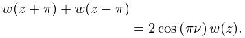
Furthermore, for each solution of (28.29.1)

28.29.13 $w(z+\pi)+w(z-\pi)=2\mathop{\cos\/}\nolimits\!\left(\pi\nu\right)w(z).$

Symbols:: $\mathop{\cos\/}\nolimits z$ : cosine function, : complex variable, $\nu$ : complex parameter and : Mathieu’s equation solution
Permalink:: http://dlmf.nist.gov/28.29.E13
Encodings:: TeX, pMML, png

A nontrivial solution is either a Floquet solution with respect to $\nu$ , or $w(z+\pi)-e^{{i\nu\pi}}w(z)$ is a Floquet solution with respect to $-\nu$ .

In the symmetric case , $w_{{\mbox{\tiny I}}}(z,\lambda)$ is an even solution and $w_{{\mbox{\tiny II}}}(z,\lambda)$ is an odd solution; compare §28.2(ii). (28.29.9) reduces to

28.29.14 $\mathop{\cos\/}\nolimits\!\left(\pi\nu\right)=w_{{\mbox{\tiny I}}}(\pi,\lambda).$

Symbols:: $\mathop{\cos\/}\nolimits z$ : cosine function, $\nu$ : complex parameter, $w_{{\mbox{\tiny I}}}(z;a,q)$ : fundamental solution and $\lambda$ : parameter
Permalink:: http://dlmf.nist.gov/28.29.E14
Encodings:: TeX, pMML, png

The cases $\nu=0$ and $\nu=1$ split into four subcases as in (28.2.21) and (28.2.22). The $\pi$ -periodic or $\pi$ -antiperiodic solutions are multiples of $w_{{\mbox{\tiny I}}}(z,\lambda),w_{{\mbox{\tiny II}}}(z,\lambda)$ , respectively.

For details and proofs see Magnus and Winkler (1966, §1.3).

§28.29(iii) Discriminant and Eigenvalues in the Real Case

Notes:: See Magnus and Winkler (1966, pp. 11–36 and §2.4).
Keywords:: Hill’s equation, discriminant
Permalink:: http://dlmf.nist.gov/28.29.iii

is assumed to be real-valued throughout this subsection.

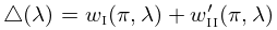
The function

28.29.15 $\bigtriangleup(\lambda)=w_{{\mbox{\tiny I}}}(\pi,\lambda)+w_{{\mbox{\tiny II}}% }^{{\prime}}(\pi,\lambda)$

Symbols:: $w_{{\mbox{\tiny I}}}(z;a,q)$ : fundamental solution, $w_{{\mbox{\tiny II}}}(z;a,q)$ : fundamental solution and $\lambda$ : parameter
Permalink:: http://dlmf.nist.gov/28.29.E15
Encodings:: TeX, pMML, png

is called the discriminant of (28.29.1). It is an entire function of $\lambda$ . Its order of growth for $|\lambda|\to\infty$ is exactly $\tfrac{1}{2}$ ; see Magnus and Winkler (1966, Chapter II, pp. 19–28).

For a given $\nu$ , the characteristic equation $\bigtriangleup(\lambda)-2\mathop{\cos\/}\nolimits\!\left(\pi\nu\right)=0$ has infinitely many roots $\lambda$ . Conversely, for a given $\lambda$ , the value of $\bigtriangleup(\lambda)$ is needed for the computation of $\nu$ . For this purpose the discriminant can be expressed as an infinite determinant involving the Fourier coefficients of ; see Magnus and Winkler (1966, §2.3, pp. 28–36).

To every equation (28.29.1), there belong two increasing infinite sequences of real eigenvalues:

28.29.16 $\lambda_{n},\;n=0,1,2,\dots,\mbox{ with $\bigtriangleup(\lambda_{n})=2$},$

Symbols:: : integer and $\lambda_{n}$ : eigenvalues
Referenced by:: §28.30(i)
Permalink:: http://dlmf.nist.gov/28.29.E16
Encodings:: TeX, pMML, png

28.29.17 $\mu_{n},\;n=1,2,3,\dots,\mbox{ with $\bigtriangleup(\mu_{n})=-2$}.$

Symbols:: : integer and $\mu_{n}$ : eigenvalues
Referenced by:: §28.30(i)
Permalink:: http://dlmf.nist.gov/28.29.E17
Encodings:: TeX, pMML, png

In consequence, (28.29.1) has a solution of period $\pi$ iff $\lambda=\lambda_{n}$ , and a solution of period $2\pi$ iff $\lambda=\mu_{n}$ . Both $\lambda_{n}$ and $\mu_{n}\to\infty$ as $n\to\infty$ , and interlace according to the inequalities

28.29.18 $\lambda_{0}<\mu_{1}\leq\mu_{2}<\lambda_{1}\leq\lambda_{2}<\mu_{3}\leq\mu_{4}<% \lambda_{3}\leq\lambda_{4}<\cdots.$

Symbols:: $\lambda_{n}$ : eigenvalues and $\mu_{n}$ : eigenvalues
Referenced by:: §28.30(i)
Permalink:: http://dlmf.nist.gov/28.29.E18
Encodings:: TeX, pMML, png

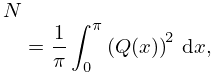
Assume that the second derivative of in (28.29.1) exists and is continuous. Then with

28.29.19 $N=\frac{1}{\pi}\int_{0}^{\pi}\left(Q(x)\right)^{2}dx,$

Symbols:: : differential of , $\int$ : integral, : real variable, : function and
Permalink:: http://dlmf.nist.gov/28.29.E19
Encodings:: TeX, pMML, png

we have for $m\to\infty$

28.29.20

$\mu_{{2m-1}}-(2m-1)^{2}-\dfrac{N}{(4m)^{2}}=\mathop{o\/}\nolimits\!\left(m^{{-% 2}}\right),$

$\mu_{{2m}}-(2m-1)^{2}-\dfrac{N}{(4m)^{2}}=\mathop{o\/}\nolimits\!\left(m^{{-2}% }\right),$

Symbols:: $\mathop{o\/}\nolimits\!\left(x\right)$ : order less than, : integer, $\mu_{n}$ : eigenvalues and
Permalink:: http://dlmf.nist.gov/28.29.E20
Encodings:: TeX, TeX, pMML, pMML, png, png

28.29.21

$\lambda_{{2m-1}}-(2m)^{2}-\dfrac{N}{(4m)^{2}}=\mathop{o\/}\nolimits\!\left(m^{% {-2}}\right),$

$\lambda_{{2m}}-(2m)^{2}-\dfrac{N}{(4m)^{2}}=\mathop{o\/}\nolimits\!\left(m^{{-% 2}}\right).$

Symbols:: $\mathop{o\/}\nolimits\!\left(x\right)$ : order less than, : integer, $\lambda_{n}$ : eigenvalues and
Permalink:: http://dlmf.nist.gov/28.29.E21
Encodings:: TeX, TeX, pMML, pMML, png, png

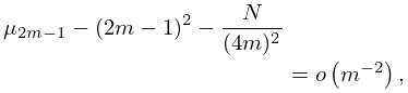
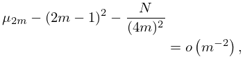
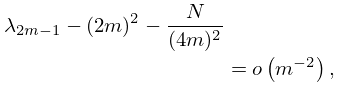
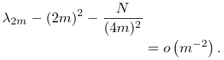
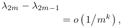
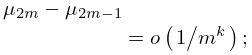
If has continuous derivatives, then as $m\to\infty$

28.29.22

$\lambda_{{2m}}-\lambda_{{2m-1}}=\mathop{o\/}\nolimits\!\left(\ifrac{1}{m^{k}}% \right),$

$\mu_{{2m}}-\mu_{{2m-1}}=\mathop{o\/}\nolimits\!\left(\ifrac{1}{m^{k}}\right);$

Symbols:: $\mathop{o\/}\nolimits\!\left(x\right)$ : order less than, : integer, $\lambda_{n}$ : eigenvalues, $\mu_{n}$ : eigenvalues and : number
Permalink:: http://dlmf.nist.gov/28.29.E22
Encodings:: TeX, TeX, pMML, pMML, png, png

see Hochstadt (1963).

For further results, especially when is analytic in a strip, see Weinstein and Keller (1987).

© 2010–2013 NIST / Privacy Policy / Disclaimer / Feedback; Version 1.0.6; Release date 2013-05-06 Math-Image version (See MathML) . A Printed Companionis available. 28.28 Integrals, Integral Representations, and Integral Equations 28.30 Expansions in Series of Eigenfunctions

§28.29 Definitions and Basic Properties

Contents

§28.29(i) Hill’s Equation

§28.29(ii) Floquet’s Theorem and the Characteristic Exponent

§28.29(iii) Discriminant and Eigenvalues in the Real Case