.世界杯规则大全图解『wn4.com』澳门足总杯超大比分.w6n2c9o.2022年12月1日14时53分9秒.h7j55xrv5

SearchAdvancedHelp

(0.008 seconds)

21—30 of 838 matching pages

21: 26.2 Basic Definitions

… ►Thus $231$ is the permutation $\sigma (1)=2$, $\sigma (2)=3$, $\sigma (3)=1$. … ►As an example, $\{1,1,1,2,4,4\}$ is a partition of 13. …See Table 26.2.1 for $n=0(1)50$. For the actual partitions ($\pi$) for $n=1(1)5$ see Table 26.4.1. … ►The example $\{1,1,1,2,4,4\}$ has six parts, three of which equal 1. …

22: 18.8 Differential Equations

… ►

Table 18.8.1: Classical OP’s: differential equations $A(x)f^{\prime \prime }(x)+B(x)f^{\prime }(x)+C(x)f(x)+{\lambda }_{n}f(x)=0$.

► ►►►►►►

#	$f(x)$	$A(x)$	$B(x)$	$C(x)$	${\lambda }_n$
…
9	${\mathrm{e}}^{-\frac{1}{2}{x}^2}{x}^{\alpha +\frac{1}{2}}{L}_n^{(\alpha )}\left(x^2\right)$	$1$	$0$	$-x^2+(\frac{1}{4}-{\alpha }^2)x^{-2}$	$4n+2\alpha +2$
10	${\mathrm{e}}^{-\frac{1}{2}x}{x}^{\frac{1}{2}\alpha }{L}_n^{(\alpha )}\left(x\right)$	$x$	$1$	$-\frac{1}{4}x-\frac{1}{4}{\alpha }^2{x}^{-1}$	$n+\frac{1}{2}(\alpha +1)$
11	${\mathrm{e}}^{-n^{-1}x}{x}^{\mathrm{\ell }+1}{L}_{n-\mathrm{\ell }-1}^{(2\mathrm{\ell }+1)}\left(2n^{-1}x\right)$	$1$	$0$	$\frac{2}{x}-\frac{\mathrm{\ell }(\mathrm{\ell }+1)}{x^2}$	$-\frac{1}{n^2}$
12	$H_n\left(x\right)$	$1$	$-2x$	$0$	$2n$
…

►

►Item 11 of Table 18.8.1 yields (18.39.36) for $Z=1$.

23: 8.26 Tables

… ►

Zhang and Jin (1996, Table 3.8) tabulates $\gamma (a,x)$ for $a=0.5,1,3,5,10,25,50,100$, $x=0(.1)1(1)3,5(5)30,50,100$ to 8D or 8S.

… ►

Zhang and Jin (1996, Table 3.9) tabulates $I_x(a,b)$ for $x=0(.05)1$, $a=0.5,1,3,5,10$, $b=1,10$ to 8D.

… ►

Chiccoli et al. (1988) presents a short table of $E_p\left(x\right)$ for $p=-\frac{9}{2}(1)-\frac{1}{2}$, $0\le x\le 200$ to 14S.

►

Pagurova (1961) tabulates $E_n\left(x\right)$ for $n=0(1)20$, $x=0(.01)2(.1)10$ to 4-9S; ${\mathrm{e}}^x{E}_n\left(x\right)$ for $n=2(1)10$, $x=10(.1)20$ to 7D; ${\mathrm{e}}^x{E}_p\left(x\right)$ for $p=0(.1)1$, $x=0.01(.01)7(.05)12(.1)20$ to 7S or 7D.

►

Stankiewicz (1968) tabulates $E_n\left(x\right)$ for $n=1(1)10$, $x=0.01(.01)5$ to 7D.

…

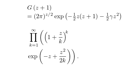
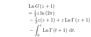
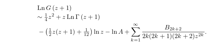
24: 5.17 Barnes’ $G$-Function (Double Gamma Function)

… ►

$G\left(1\right)=1,$

… ►

5.17.3 $$G\left(z+1\right)={(2\pi )}^{z/2}\exp \left(-\frac{1}{2}z(z+1)-\frac{1}{2}\gamma z^2\right)\prod _{k=1}^{\mathrm{\infty }}\left({\left(1+\frac{z}{k}\right)}^k\exp \left(-z+\frac{z^2}{2k}\right)\right).$$

ⓘ

Symbols:

$G\left(z\right)$: Barnes’ $G$-function (or double gamma function), $\gamma$: Euler’s constant, $\pi$: the ratio of the circumference of a circle to its diameter, $\exp z$: exponential function, $k$: nonnegative integer and $z$: complex variable

Permalink:

http://dlmf.nist.gov/5.17.E3

Encodings:

pMML, png, TeX

See also:

Annotations for §5.17 and Ch.5

►

5.17.4 $$\mathrm{Ln}G\left(z+1\right)=\frac{1}{2}z\ln \left(2\pi \right)-\frac{1}{2}z(z+1)+z\mathrm{Ln}\mathrm{\Gamma }\left(z+1\right)-{\int }_0^z\mathrm{Ln}\mathrm{\Gamma }\left(t+1\right)dt.$$

ⓘ

Symbols:

$G\left(z\right)$: Barnes’ $G$-function (or double gamma function), $\mathrm{\Gamma }\left(z\right)$: gamma function, $\pi$: the ratio of the circumference of a circle to its diameter, $dx$: differential of $x$ , $\int$: integral, $\mathrm{Ln}z$: general logarithm function, $\ln z$: principal branch of logarithm function and $z$: complex variable

Permalink:

http://dlmf.nist.gov/5.17.E4

Encodings:

pMML, png, TeX

See also:

Annotations for §5.17 and Ch.5

… ►

5.17.5 $$\mathrm{Ln}G\left(z+1\right)\sim \frac{1}{4}{z}^2+z\mathrm{Ln}\mathrm{\Gamma }\left(z+1\right)-\left(\frac{1}{2}z(z+1)+\frac{1}{12}\right)\ln z-\ln A+\sum _{k=1}^{\mathrm{\infty }}\frac{B_{2k+2}}{2k(2k+1)(2k+2)z^{2k}}.$$

ⓘ

Symbols:

$G\left(z\right)$: Barnes’ $G$-function (or double gamma function), $B_n$: Bernoulli numbers, $\mathrm{\Gamma }\left(z\right)$: gamma function, $\sim$: Poincaré asymptotic expansion, $\mathrm{Ln}z$: general logarithm function, $\ln z$: principal branch of logarithm function, $k$: nonnegative integer, $z$: complex variable and $A$: Glaisher’s constant

Referenced by:

§5.17, §5.17, Erratum (V1.0.7) for Equation (5.17.5), Erratum (V1.1.11) for Equation (5.17.5)

Permalink:

http://dlmf.nist.gov/5.17.E5

Encodings:

pMML, png, TeX

Errata (effective with 1.1.11):

For consistency we have replaced $\mathrm{Ln}z$ by $\ln z$.

Errata (effective with 1.0.7):

Originally the term $z\mathrm{Ln}\mathrm{\Gamma }\left(z+1\right)$ was incorrectly stated as $z\mathrm{\Gamma }\left(z+1\right)$. (This error was reported subsequently by Nick Jones on December 11, 2013.)

Reported 2013-08-01 by Gergő Nemes

See also:

Annotations for §5.17 and Ch.5

… ►

5.17.7 $$C=\underset{n\to \mathrm{\infty }}{lim}\left(\sum _{k=1}^{n}k\ln k-\left(\frac{1}{2}{n}^2+\frac{1}{2}n+\frac{1}{12}\right)\ln n+\frac{1}{4}{n}^2\right)=\frac{\gamma +\ln \left(2\pi \right)}{12}-\frac{{\zeta }^{\prime }\left(2\right)}{2{\pi }^2}=\frac{1}{12}-{\zeta }^{\prime }\left(-1\right),$$

ⓘ

Symbols:

$\gamma$: Euler’s constant, $\zeta \left(s\right)$: Riemann zeta function, $\pi$: the ratio of the circumference of a circle to its diameter, $\ln z$: principal branch of logarithm function, $n$: nonnegative integer, $k$: nonnegative integer and $C$: log of Glaisher’s Constant

Referenced by:

§5.17

Permalink:

http://dlmf.nist.gov/5.17.E7

Encodings:

pMML, png, TeX

See also:

Annotations for §5.17 and Ch.5

…

25: 26.9 Integer Partitions: Restricted Number and Part Size

… ►The conjugate to the example in Figure 26.9.1 is $6+5+4+2+1+1+1$. … ►It is also equal to the number of lattice paths from $(0,0)$ to $(m,k)$ that have exactly $n$ vertices $(h,j)$, $1\le h\le m$, $1\le j\le k$, above and to the left of the lattice path. … ►

$p_3\left(n\right)=1+\lfloor {\displaystyle \frac{n^2+6n}{12}}\rfloor .$

… ►It is also assumed everywhere that . … ►Also, when …

26: Bibliography G

… ►

Algorithm 939: computation of the Marcum Q-function. ACM Trans. Math. Softw. 40 (3), pp. 20:1–20:21.

ⓘ

Notes:

Includes Fortran program claiming 12S accuracy

External Links:

ISSN 0098-3500, Link, Document, MathReview Entry, ZentralBlatt

Referenced by:

3rd item, §10.77(ix).

Encodings:

BibTeX

… ►

Fourier transforms related to a root system of rank 1. Transform. Groups 12 (1), pp. 77–116.

ⓘ

External Links:

ISSN 1083-4362, Link, MathReview (Genkai Zhang), ZentralBlatt

Referenced by:

§18.28(xi), §18.38(iii).

Encodings:

BibTeX

… ►

The solutions of Painlevé’s fifth equation. Differ. Uravn. 12 (4), pp. 740–742 (Russian).

ⓘ

Notes:

In Russian. English translation: Differential Equations 12(4), pp. 519–521 (1977)

External Links:

MathReview (Z. Nehari), ZentralBlatt

Referenced by:

§32.7(v).

Encodings:

BibTeX

►

One-parameter systems of solutions of Painlevé equations. Differ. Uravn. 14 (12), pp. 2131–2135 (Russian).

ⓘ

Notes:

In Russian. English translation: Differential Equations 14(12), pp. 1510–1513 (1979)

External Links:

ISSN 0374-0641, MathReview (M. Tvrdý), ZentralBlatt

Referenced by:

§32.10(i), §32.10(ii), §32.10(iii), §32.7(iv).

Encodings:

BibTeX

… ►

Algorithm 300: Coulomb wave functions. Comm. ACM 10 (4), pp. 244–245.

ⓘ

Notes:

For remarks see same journal 12(1969), p. 692 and 16(1973), pp. 308-309 and for certification see same journal 12(1969), pp. 279-280.

External Links:

ISSN 0001-0782, Document

Referenced by:

§33.26(ii).

Encodings:

BibTeX

…

27: 28.6 Expansions for Small $q$

… ►Leading terms of the of the power series for $m=7,8,9,\mathrm{\dots }$ are: … ►The coefficients of the power series of $a_{2n}\left(q\right)$, $b_{2n}\left(q\right)$ and also $a_{2n+1}\left(q\right)$, $b_{2n+1}\left(q\right)$ are the same until the terms in $q^{2n-2}$ and $q^{2n}$, respectively. … ►Numerical values of the radii of convergence ${\rho }_n^{(j)}$ of the power series (28.6.1)–(28.6.14) for $n=0,1,\mathrm{\dots },9$ are given in Table 28.6.1. Here $j=1$ for $a_{2n}\left(q\right)$, $j=2$ for $b_{2n+2}\left(q\right)$, and $j=3$ for $a_{2n+1}\left(q\right)$ and $b_{2n+1}\left(q\right)$. 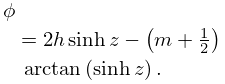… ►where $k$ is the unique root of the equation $2E\left(k\right)=K\left(k\right)$ in the interval $(0,1)$, and $k^{\prime }=\sqrt{1-k^2}$. …

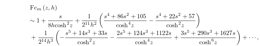
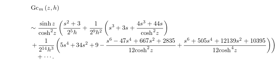
28: 28.26 Asymptotic Approximations for Large $q$

… ►

28.26.2 $$\mathrm{i}{\mathrm{Ms}}_{m+1}^{(3)}(z,h)=\frac{{\mathrm{e}}^{\mathrm{i}\varphi }}{{(\pi h\cosh z)}^{1/2}}\left({\mathrm{Fs}}_m(z,h)-\mathrm{i}{\mathrm{Gs}}_m(z,h)\right),$$

ⓘ

Symbols:

$\pi$: the ratio of the circumference of a circle to its diameter, $\mathrm{e}$: base of natural logarithm, $\cosh z$: hyperbolic cosine function, $\mathrm{i}$: imaginary unit, ${\mathrm{Ms}}_n^{(j)}(z,h)$: radial Mathieu function, $m$: integer, $h$: parameter, $z$: complex variable and $\varphi$

A&S Ref:

20.9.7 (in slightly different notation)

Permalink:

http://dlmf.nist.gov/28.26.E2

Encodings:

pMML, png, TeX

See also:

Annotations for §28.26(i), §28.26 and Ch.28

… ►

28.26.3 $$\varphi =2h\sinh z-\left(m+\frac{1}{2}\right)\arctan \left(\sinh z\right).$$

ⓘ

Symbols:

$\sinh z$: hyperbolic sine function, $\arctan z$: arctangent function, $m$: integer, $h$: parameter, $z$: complex variable and $\varphi$

A&S Ref:

20.9.8 (in slightly different notation)

Permalink:

http://dlmf.nist.gov/28.26.E3

Encodings:

pMML, png, TeX

See also:

Annotations for §28.26(i), §28.26 and Ch.28

►Then as $h\to +\mathrm{\infty }$ with fixed $z$ in $\mathrm{\Re }z>0$ and fixed $s=2m+1$, ►

28.26.4 $${\mathrm{Fc}}_m(z,h)\sim 1+\frac{s}{8h{\cosh }^{2}z}+\frac{1}{2^{11}{h}^2}\left(\frac{s^4+86s^2+105}{{\cosh }^{4}z}-\frac{s^4+22s^2+57}{{\cosh }^{2}z}\right)+\frac{1}{2^{14}{h}^3}\left(-\frac{s^5+14s^3+33s}{{\cosh }^{2}z}-\frac{2s^5+124s^3+1122s}{{\cosh }^{4}z}+\frac{3s^5+290s^3+1627s}{{\cosh }^{6}z}\right)+\mathrm{\cdots },$$

ⓘ

Symbols:

$\sim$: Poincaré asymptotic expansion, $\cosh z$: hyperbolic cosine function, $m$: integer, $h$: parameter and $z$: complex variable

A&S Ref:

20.9.9 (in slightly different notation)

Referenced by:

§28.26(i)

Permalink:

http://dlmf.nist.gov/28.26.E4

Encodings:

pMML, png, TeX

See also:

Annotations for §28.26(i), §28.26 and Ch.28

►

28.26.5 $${\mathrm{Gc}}_m(z,h)\sim \frac{\sinh z}{{\cosh }^{2}z}\left(\frac{s^2+3}{2^{5}h}+\frac{1}{2^9{h}^2}\left(s^3+3s+\frac{4s^3+44s}{{\cosh }^{2}z}\right)+\frac{1}{2^{14}{h}^3}\left(5s^4+34s^2+9-\frac{s^6-47s^4+667s^2+2835}{12{\cosh }^{2}z}+\frac{s^6+505s^4+12139s^2+10395}{12{\cosh }^{4}z}\right)\right)+\mathrm{\cdots }.$$

ⓘ

Symbols:

$\sim$: Poincaré asymptotic expansion, $\cosh z$: hyperbolic cosine function, $\sinh z$: hyperbolic sine function, $m$: integer, $h$: parameter and $z$: complex variable

A&S Ref:

20.9.10 (in slightly different notation)

Referenced by:

§28.26(i)

Permalink:

http://dlmf.nist.gov/28.26.E5

Encodings:

pMML, png, TeX

See also:

Annotations for §28.26(i), §28.26 and Ch.28

…

29: 5.23 Approximations

… ►Cody and Hillstrom (1967) gives minimax rational approximations for $\ln \mathrm{\Gamma }\left(x\right)$ for the ranges $0.5\le x\le 1.5$, $1.5\le x\le 4$, $4\le x\le 12$; precision is variable. Hart et al. (1968) gives minimax polynomial and rational approximations to $\mathrm{\Gamma }\left(x\right)$ and $\ln \mathrm{\Gamma }\left(x\right)$ in the intervals $0\le x\le 1$, $8\le x\le 1000$, $12\le x\le 1000$; precision is variable. … ►Luke (1969b) gives the coefficients to 20D for the Chebyshev-series expansions of $\mathrm{\Gamma }\left(1+x\right)$, $1/\mathrm{\Gamma }\left(1+x\right)$, $\mathrm{\Gamma }\left(x+3\right)$, $\ln \mathrm{\Gamma }\left(x+3\right)$, $\psi \left(x+3\right)$, and the first six derivatives of $\psi \left(x+3\right)$ for $0\le x\le 1$. …Clenshaw (1962) also gives 20D Chebyshev-series coefficients for $\mathrm{\Gamma }\left(1+x\right)$ and its reciprocal for $0\le x\le 1$. …

30: 16.12 Products

… ►

16.12.1 $${}_0{}^{}F_1^{}(-;a;z){}_0{}^{}F_1^{}(-;b;z)={}_2{}^{}F_3^{}(\genfrac{}{}{0pt}{}{\frac{1}{2}(a+b),\frac{1}{2}(a+b-1)}{a,b,a+b-1};4z).$$

ⓘ

Symbols:

${}_p{}^{}F_q^{}(a_1,\mathrm{\dots },a_p;b_1,\mathrm{\dots },b_q;z)$ or ${}_p{}^{}F_q^{}(\genfrac{}{}{0pt}{}{a_1,\mathrm{\dots },a_p}{b_1,\mathrm{\dots },b_q};z)$: alternatively ${}_p{}^{}F_q^{}(𝐚;𝐛;z)$ or ${}_p{}^{}F_q^{}(\genfrac{}{}{0pt}{}{𝐚}{𝐛};z)$
generalized hypergeometric function, $z$: complex variable, $a,a_1,\mathrm{\dots },a_p$: real or complex parameters and $b,b_1,\mathrm{\dots },b_q$: real or complex parameters

Referenced by:

(10.8.3), §10.8, §10.8, §16.12, Erratum (V1.0.17) for Section 10.8

Permalink:

http://dlmf.nist.gov/16.12.E1

Encodings:

pMML, png, TeX

See also:

Annotations for §16.12 and Ch.16

… ►

16.12.2 $${\left({}_2{}^{}F_1^{}(\genfrac{}{}{0pt}{}{a,b}{a+b+\frac{1}{2}};z)\right)}^2={}_3{}^{}F_2^{}(\genfrac{}{}{0pt}{}{2a,2b,a+b}{a+b+\frac{1}{2},2a+2b};z).$$

ⓘ

Symbols:

${}_2{}^{}F_1^{}(a,b;c;z)$: $=F(a,b;c;z)$ notation for Gauss’ hypergeometric function, ${}_p{}^{}F_q^{}(a_1,\mathrm{\dots },a_p;b_1,\mathrm{\dots },b_q;z)$ or ${}_p{}^{}F_q^{}(\genfrac{}{}{0pt}{}{a_1,\mathrm{\dots },a_p}{b_1,\mathrm{\dots },b_q};z)$: alternatively ${}_p{}^{}F_q^{}(𝐚;𝐛;z)$ or ${}_p{}^{}F_q^{}(\genfrac{}{}{0pt}{}{𝐚}{𝐛};z)$
generalized hypergeometric function, $z$: complex variable, $a,a_1,\mathrm{\dots },a_p$: real or complex parameters and $b,b_1,\mathrm{\dots },b_q$: real or complex parameters

Referenced by:

§16.12, §17.9(iii), Erratum (V1.1.12) for Subsection 17.9(iii)

Permalink:

http://dlmf.nist.gov/16.12.E2

Encodings:

pMML, png, TeX

See also:

Annotations for §16.12 and Ch.16

… ►

16.12.3 $${\left({}_2{}^{}F_1^{}(\genfrac{}{}{0pt}{}{a,b}{c};z)\right)}^2=\sum _{k=0}^{\mathrm{\infty }}\frac{{\left(2a\right)}_k{\left(2b\right)}_k{\left(c-\frac{1}{2}\right)}_k}{{\left(c\right)}_k{\left(2c-1\right)}_{k}k!}{}_4{}^{}F_3^{}(\genfrac{}{}{0pt}{}{-\frac{1}{2}k,\frac{1}{2}(1-k),a+b-c+\frac{1}{2},\frac{1}{2}}{a+\frac{1}{2},b+\frac{1}{2},\frac{3}{2}-k-c};1)z^k,$$ .

ⓘ

Symbols:

${}_2{}^{}F_1^{}(a,b;c;z)$: $=F(a,b;c;z)$ notation for Gauss’ hypergeometric function, ${}_p{}^{}F_q^{}(a_1,\mathrm{\dots },a_p;b_1,\mathrm{\dots },b_q;z)$ or ${}_p{}^{}F_q^{}(\genfrac{}{}{0pt}{}{a_1,\mathrm{\dots },a_p}{b_1,\mathrm{\dots },b_q};z)$: alternatively ${}_p{}^{}F_q^{}(𝐚;𝐛;z)$ or ${}_p{}^{}F_q^{}(\genfrac{}{}{0pt}{}{𝐚}{𝐛};z)$
generalized hypergeometric function, ${\left(a\right)}_n$: Pochhammer’s symbol (or shifted factorial), $!$: factorial (as in $n!$), $z$: complex variable, $a,a_1,\mathrm{\dots },a_p$: real or complex parameters and $b,b_1,\mathrm{\dots },b_q$: real or complex parameters

Referenced by:

§16.12

Permalink:

http://dlmf.nist.gov/16.12.E3

Encodings:

pMML, png, TeX

See also:

Annotations for §16.12 and Ch.16

…