.2014年世界杯朝鲜战绩『网址:mxsty.cc』.世界杯1998假球-m6q3s2-2022年11月30日9时27分4秒

(0.005 seconds)

21—30 of 539 matching pages

21: Bibliography K

… ►

E. G. Kalnins, W. Miller, and P. Winternitz (1976) The group

{\rm{O}}(4)

, separation of variables and the hydrogen atom. SIAM J. Appl. Math. 30 (4), pp. 630–664.

ⓘ

External Links:: Document, MathReview (Anthony J. Bracken), ZentralBlatt
Referenced by:: §31.17(i).
Encodings:: BibTeX

… ►

G. A. Kalugin, D. J. Jeffrey, and R. M. Corless (2012) Bernstein, Pick, Poisson and related integral expressions for Lambert

W

. Integral Transforms Spec. Funct. 23 (11), pp. 817–829.

ⓘ

External Links:: ISSN 1065-2469, Document, Link, MathReview (Ross C. McPhedran), ZentralBlatt
Referenced by:: §4.13.
Encodings:: BibTeX

… ►

E. L. Kaplan (1948) Auxiliary table for the incomplete elliptic integrals. J. Math. Physics 27, pp. 11–36.

ⓘ

External Links:: MathReview (S. C. van Veen), ZentralBlatt
Referenced by:: §19.12.
Encodings:: BibTeX

… ►

K. S. Kölbig (1968) Algorithm 327: Dilogarithm [S22]. Comm. ACM 11 (4), pp. 270–271.

ⓘ

Notes:: Includes Algol program, maximum accuracy 12D.
External Links:: ISSN 0001-0782, Document
Referenced by:: §25.21(v).
Encodings:: BibTeX

… ►

T. H. Koornwinder (1989) Meixner-Pollaczek polynomials and the Heisenberg algebra. J. Math. Phys. 30 (4), pp. 767–769.

ⓘ

External Links:: ISSN 0022-2488, Document, MathReview, ZentralBlatt
Referenced by:: §18.21(ii).
Encodings:: BibTeX

…

B. R. Fabijonas, D. W. Lozier, and F. W. J. Olver (2004) Computation of complex Airy functions and their zeros using asymptotics and the differential equation. ACM Trans. Math. Software 30 (4), pp. 471–490.

ⓘ

External Links:: ISSN 0098-3500, Document, MathReview, ZentralBlatt
Referenced by:: §9.17(ii), §9.17(v), §9.8(iv).
Encodings:: BibTeX

… ►

B. R. Fabijonas (2004) Algorithm 838: Airy functions. ACM Trans. Math. Software 30 (4), pp. 491–501.

ⓘ

Notes:: Single- and double-precision Fortran, maximum accuracy 32S.
External Links:: ISSN 0098-3500, Document, Code, MathReview Entry, ZentralBlatt
Referenced by:: 3rd item, 2nd item, 1st item.
Encodings:: BibTeX

… ►

N. Fleury and A. Turbiner (1994) Polynomial relations in the Heisenberg algebra. J. Math. Phys. 35 (11), pp. 6144–6149.

ⓘ

External Links:: ISSN 0022-2488, Document, MathReview (Shao-Ming Fei), ZentralBlatt
Referenced by:: §13.3(ii), §15.5(i), §16.3(i).
Encodings:: BibTeX

… ►

A. S. Fokas and M. J. Ablowitz (1982) On a unified approach to transformations and elementary solutions of Painlevé equations. J. Math. Phys. 23 (11), pp. 2033–2042.

ⓘ

External Links:: ISSN 0022-2488, Document, MathReview (Hélène Airault), ZentralBlatt
Referenced by:: §32.13(i), §32.7(i), §32.7(iii).
Encodings:: BibTeX

… ►

L. W. Fullerton (1972) Algorithm 435: Modified incomplete gamma function. Comm. ACM 15 (11), pp. 993–995.

ⓘ

Notes:: Includes Fortran code. For a Remark see ACM Trans. Math. Software 4 (1978), no. 3, pp. 296–304.
External Links:: ISSN 0001-0782, Document, Remark
Referenced by:: §8.28(ii).
Encodings:: BibTeX

…

23: Bibliography

… ►

M. Abramowitz (1949) Asymptotic expansions of spheroidal wave functions. J. Math. Phys. Mass. Inst. Tech. 28, pp. 195–199.

ⓘ

External Links:: MathReview (J. G. van der Corput), ZentralBlatt
Referenced by:: §30.9(iii).
Encodings:: BibTeX

… ►

S. Ahmed and M. E. Muldoon (1980) On the zeros of confluent hypergeometric functions. III. Characterization by means of nonlinear equations. Lett. Nuovo Cimento (2) 29 (11), pp. 353–358.

ⓘ

External Links:: ISSN 0024-1318, MathReview (James M. Horner)
Referenced by:: §13.9(i).
Encodings:: BibTeX

… ►

V. I. Arnol’d (1974) Normal forms of functions in the neighborhood of degenerate critical points. Uspehi Mat. Nauk 29 (2(176)), pp. 11–49 (Russian).

ⓘ

Notes:: Collection of articles dedicated to the memory of Ivan Georgievič Petrovskiĭ (1901–1973), I. In Russian. English translation: Russian Math. Surveys, 29(1974), no. 2, pp. 10–50.
External Links:: Document, MathReview (G. R. Belickii), ZentralBlatt
Referenced by:: §36.2(i).
Encodings:: BibTeX

►

V. I. Arnol’d (1975) Critical points of smooth functions, and their normal forms. Uspehi Mat. Nauk 30 (5(185)), pp. 3–65 (Russian).

ⓘ

Notes:: In Russian. English translation: Russian Math. Surveys, 30(1975), no. 5, pp. 1–75.
External Links:: Document, MathReview (D. Siersma), ZentralBlatt
Referenced by:: §36.2(i), Ch.36.
Encodings:: BibTeX

… ►

R. Askey (1980) Some basic hypergeometric extensions of integrals of Selberg and Andrews. SIAM J. Math. Anal. 11 (6), pp. 938–951.

ⓘ

External Links:: ISSN 0036-1410, Document, MathReview (W. A. Al-Salam), ZentralBlatt
Referenced by:: §17.13, §17.13.
Encodings:: BibTeX

…

24: 34.6 Definition: $\mathit{9j}$ Symbol

… ►

34.6.1

\begin{Bmatrix}j_{11}&j_{12}&j_{13}\\ j_{21}&j_{22}&j_{23}\\ j_{31}&j_{32}&j_{33}\end{Bmatrix}=\sum_{\mbox{\scriptsize all }m_{rs}}\begin{% pmatrix}j_{11}&j_{12}&j_{13}\\ m_{11}&m_{12}&m_{13}\end{pmatrix}\begin{pmatrix}j_{21}&j_{22}&j_{23}\\ m_{21}&m_{22}&m_{23}\end{pmatrix}\begin{pmatrix}j_{31}&j_{32}&j_{33}\\ m_{31}&m_{32}&m_{33}\end{pmatrix}\*\begin{pmatrix}j_{11}&j_{21}&j_{31}\\ m_{11}&m_{21}&m_{31}\end{pmatrix}\begin{pmatrix}j_{12}&j_{22}&j_{32}\\ m_{12}&m_{22}&m_{32}\end{pmatrix}\begin{pmatrix}j_{13}&j_{23}&j_{33}\\ m_{13}&m_{23}&m_{33}\end{pmatrix},

ⓘ

Defines:: $\begin{Bmatrix}\NVar{j_{11}}&\NVar{j_{12}}&\NVar{j_{13}}\\ \NVar{j_{21}}&\NVar{j_{22}}&\NVar{j_{23}}\\ \NVar{j_{31}}&\NVar{j_{32}}&\NVar{j_{33}}\end{Bmatrix}$ : $\mathit{9j}$ symbol
Symbols:: $\begin{pmatrix}\NVar{j_{1}}&\NVar{j_{2}}&\NVar{j_{3}}\\ \NVar{m_{1}}&\NVar{m_{2}}&\NVar{m_{3}}\end{pmatrix}$ : $\mathit{3j}$ symbol, $j,j_{r}$ : non-negative integers or non-negative integers plus one half., $r$ : nonnegative integer and $s$ : integer
Permalink:: http://dlmf.nist.gov/34.6.E1
Encodings:: pMML, png, TeX
See also:: Annotations for §34.6 and Ch.34

►

34.6.2

\begin{Bmatrix}j_{11}&j_{12}&j_{13}\\ j_{21}&j_{22}&j_{23}\\ j_{31}&j_{32}&j_{33}\end{Bmatrix}=\sum_{j}(-1)^{2j}(2j+1)\begin{Bmatrix}j_{11}% &j_{21}&j_{31}\\ j_{32}&j_{33}&j\end{Bmatrix}\begin{Bmatrix}j_{12}&j_{22}&j_{32}\\ j_{21}&j&j_{23}\end{Bmatrix}\begin{Bmatrix}j_{13}&j_{23}&j_{33}\\ j&j_{11}&j_{12}\end{Bmatrix}.

ⓘ

Symbols:: $\begin{Bmatrix}\NVar{j_{11}}&\NVar{j_{12}}&\NVar{j_{13}}\\ \NVar{j_{21}}&\NVar{j_{22}}&\NVar{j_{23}}\\ \NVar{j_{31}}&\NVar{j_{32}}&\NVar{j_{33}}\end{Bmatrix}$ : $\mathit{9j}$ symbol, $\begin{Bmatrix}\NVar{j_{1}}&\NVar{j_{2}}&\NVar{j_{3}}\\ \NVar{l_{1}}&\NVar{l_{2}}&\NVar{l_{3}}\end{Bmatrix}$ : $\mathit{6j}$ symbol and $j,j_{r}$ : non-negative integers or non-negative integers plus one half.
Referenced by:: §34.13
Permalink:: http://dlmf.nist.gov/34.6.E2
Encodings:: pMML, png, TeX
See also:: Annotations for §34.6 and Ch.34

…

25: Bibliography E

… ►

C. Eckart (1930) The penetration of a potential barrier by electrons. Phys. Rev. 35 (11), pp. 1303–1309.

ⓘ

External Links:: Document, ZentralBlatt
Referenced by:: §15.18.
Encodings:: BibTeX

… ►

M. Eichler and D. Zagier (1982) On the zeros of the Weierstrass

\wp

-function. Math. Ann. 258 (4), pp. 399–407.

ⓘ

External Links:: ISSN 0025-5831, Document, MathReview (Toyokazu Hiramatsu), ZentralBlatt
Referenced by:: §23.13.
Encodings:: BibTeX

… ►

A. Erdélyi, W. Magnus, F. Oberhettinger, and F. G. Tricomi (1953a) Higher Transcendental Functions. Vol. I. McGraw-Hill Book Company, Inc., New York-Toronto-London.

ⓘ

Notes:: Reprinted by Robert E. Krieger Publishing Co. Inc., 1981. Table errata: Math. Comp. v. 65 (1996), no. 215, p. 1385, v. 41 (1983), no. 164, p. 778, v. 30 (1976), no. 135, p. 675, v. 25 (1971), no. 115, p. 635, v. 25 (1971), no. 113, p. 199, v. 24 (1970), no. 112, p. 999, v. 24 (1970), no. 110, p. 504, v. 17 (1963), no. 84, p. 485.
External Links:: MathReview (E. T. Copson), ZentralBlatt
Referenced by:: §13.1, §13.10(ii), §13.10(iv), §13.12, §13.13(i), §13.16(ii), §13.16(iii), §13.23(i), §13.23(ii), §13.25, §13.4(i), §13.4(ii), §13.9(i), §13.9(ii), Ch.13, §14.1, §14.10, §14.12(ii), §14.12(i), §14.12(ii), §14.13, §14.13, §14.17(ii), §14.17(iv), §14.18(ii), §14.18(iii), §14.18(iv), §14.19(i), §14.19(ii), §14.19(iii), §14.19(iv), §14.20(v), §14.21(iii), §14.25, §14.28(i), §14.28(ii), §14.3(iii), §14.3(iii), §14.3(iv), §14.5(iii), §14.5(iv), §14.6(i), §14.6(ii), §14.7(iv), §14.8(i), §14.8(ii), Ch.14, §15.16, §15.4(iii), §15.5(i), §15.6, §15.8(v), §15.8(ii), §15.8(v), §15.9(iii), Ch.15, §16.12, §16.12, §16.13, §16.14(i), §16.14(ii), (16.15.3), §16.15, §16.16(i), §16.16(ii), §16.18, §16.20, §16.20, §16.21, §16.4(ii), §16.5, §16.6, Ch.16, §19.21(i), §19.28, §19.5, §24.16(iii), §24.5(i), §24.7(i), §24.7(ii), §24.8(i), Ch.24, (25.11.12), (25.11.18), (25.11.29), (25.11.30), (25.12.12), (25.12.13), (25.14.1), (25.14.4), (25.14.5), (25.14.6), §25.14(i), §25.14(i), §25.14(ii), §25.14(ii), §25.14, (25.5.1), (25.5.10), (25.5.11), (25.5.20), (25.5.21), (25.5.3), (25.5.8), (25.5.9), §25.5(i), §25.5(iii), §25.5, (25.8.5), (25.8.6), §25.8, Ch.25, §5.7(i), Ch.5, Notations P, Notations P, Notations Q.
Encodings:: BibTeX

►

A. Erdélyi, W. Magnus, F. Oberhettinger, and F. G. Tricomi (1953b) Higher Transcendental Functions. Vol. II. McGraw-Hill Book Company, Inc., New York-Toronto-London.

ⓘ

Notes:: Reprinted by Robert E. Krieger Publishing Co. Inc., 1981. Table errata: Math. Comp. v. 41 (1983), no. 164, p. 778, v. 36 (1981), no. 153, p. 315, v. 30 (1976), no. 135, p. 675, v. 29 (1975), no. 130, p. 670, v. 26 (1972), no. 118, p. 598, v. 25 (1971), no. 113, p. 199, v. 24 (1970), no. 109, p. 239, v. 17 (1963), no. 84, p. 485.
External Links:: MathReview (E. T. Copson), ZentralBlatt
Referenced by:: §10.22(iv), §10.22(vi), §10.23(iii), §10.23(iii), §10.23(iv), §10.32(i), §10.32(iii), §10.32(iv), §10.43(iv), §10.43(vi), §10.44(iv), §10.60(iv), §10.9(i), §10.9(iii), §10.9(iv), §11.10(vi), §11.4(i), Ch.11, §12.12, §12.12, §12.13(i), §12.5(iv), Ch.12, §18.16(vi), (18.17.21_1), §18.17(iv), §18.17(i), §18.17(viii), (18.35.1), (18.35.2), (18.35.4_5), §18.35(i), (18.5.11_1), (18.5.11_3), §18.5(ii), §18.9(iii), §19.1, §19.10(i), §19.14(ii), (19.25.40), §19.25(vi), §19.5, §19.7(ii), §19.9(i), Ch.19, §20.9(i), §22.15(ii), §23.6(iv), Ch.23, §8.13(i), §8.14, §8.3(i), §8.4, §8.6(iii), §8.7, Ch.8, Notations P, Notations P.
Encodings:: BibTeX

… ►

L. Euler (1768) Institutiones Calculi Integralis. Opera Omnia (1), Vol. 11, pp. 110–113.

ⓘ

Referenced by:: §25.12(i).
Encodings:: BibTeX

…

26: 9.18 Tables

… ►

•

Miller (1946) tabulates $\operatorname{Ai}\left(x\right)$ , $\operatorname{Ai}'\left(x\right)$ for $x=-20(.01)2;$ $\operatorname{log}_{10}\operatorname{Ai}\left(x\right)$ , $\operatorname{Ai}'\left(x\right)/\operatorname{Ai}\left(x\right)$ for $x=0(.1)25(1)75$ ; $\operatorname{Bi}\left(x\right)$ , $\operatorname{Bi}'\left(x\right)$ for $x=-10(.1)2.5$ ; $\operatorname{log}_{10}\operatorname{Bi}\left(x\right)$ , $\operatorname{Bi}'\left(x\right)/\operatorname{Bi}\left(x\right)$ for $x=0(.1)10$ ; $M\left(x\right)$ , $N\left(x\right)$ , $\theta\left(x\right)$ , $\phi\left(x\right)$ (respectively $F(x)$ , $G(x)$ , $\chi(x)$ , $\psi(x)$ ) for $x=-80(1)-30(.1)0$ . Precision is generally 8D; slightly less for some of the auxiliary functions. Extracts from these tables are included in Abramowitz and Stegun (1964, Chapter 10), together with some auxiliary functions for large arguments.

►

•

Fox (1960, Table 3) tabulates $2\pi^{1/2}x^{1/4}\*\exp(\tfrac{2}{3}x^{3/2})\*\operatorname{Ai}\left(x\right)$ , $2\pi^{1/2}x^{-1/4}\*\exp(\tfrac{2}{3}x^{3/2})\*\operatorname{Ai}'\left(x\right)$ , $\pi^{1/2}x^{1/4}\*\exp(-\tfrac{2}{3}x^{3/2})\*\operatorname{Bi}\left(x\right)$ , and $\pi^{1/2}x^{-1/4}\*\exp(-\tfrac{2}{3}x^{3/2})\*\operatorname{Bi}'\left(x\right)$ for $\tfrac{3}{2}x^{-3/2}=0(.001)0.05$ , together with similar auxiliary functions for negative values of $x$ . Precision is 10D.

… ►

•

National Bureau of Standards (1958) tabulates $A_{0}(x)\equiv\pi\operatorname{Hi}\left(-x\right)$ and $-A_{0}^{\prime}(x)\equiv\pi\operatorname{Hi}'\left(-x\right)$ for $x=0(.01)1(.02)5(.05)11$ and $1/x=0.01(.01)0.1$ ; $\int_{0}^{x}A_{0}(t)\,\mathrm{d}t$ for $x=0.5,1(1)11$ . Precision is 8D.

… ►

•

Gil et al. (2003c) tabulates the only positive zero of $\operatorname{Gi}'\left(z\right)$ , the first 10 negative real zeros of $\operatorname{Gi}\left(z\right)$ and $\operatorname{Gi}'\left(z\right)$ , and the first 10 complex zeros of $\operatorname{Gi}\left(z\right)$ , $\operatorname{Gi}'\left(z\right)$ , $\operatorname{Hi}\left(z\right)$ , and $\operatorname{Hi}'\left(z\right)$ . Precision is 11 or 12S.

… ►

•

Smirnov (1960) tabulates $U_{1}(x,\alpha)$ , $U_{2}(x,\alpha)$ , defined by (9.13.20), (9.13.21), and also $\ifrac{\partial U_{1}(x,\alpha)}{\partial x}$ , $\ifrac{\partial U_{2}(x,\alpha)}{\partial x}$ , for $\alpha=1$ , $x=-6(.01)10$ to 5D or 5S, and also for $\alpha=\pm\tfrac{1}{4}$ , $\pm\tfrac{1}{3}$ , $\pm\tfrac{1}{2}$ , $\pm\tfrac{2}{3}$ , $\pm\tfrac{3}{4}$ , $\tfrac{5}{4}$ , $\tfrac{4}{3}$ , $\tfrac{3}{2}$ , $\tfrac{5}{3}$ , $\tfrac{7}{4}$ , 2, $x=0(.01)6$ ; 4D.

27: 18.8 Differential Equations

… ►

Table 18.8.1: Classical OP’s: differential equations

A(x)f^{\prime\prime}(x)+B(x)f^{\prime}(x)+C(x)f(x)+\lambda_{n}f(x)=0

► ►►►►►►

#	$f(x)$	$A(x)$	$B(x)$	$C(x)$	$\lambda_{n}$
…
2	$\begin{gathered}\textstyle\left(\sin\frac{1}{2}x\right)^{\alpha+\frac{1}{2}}% \left(\cos\frac{1}{2}x\right)^{\beta+\frac{1}{2}}\\ \times P^{(\alpha,\beta)}_{n}\left(\cos x\right)\end{gathered}$	$1$	$0$	$\dfrac{\tfrac{1}{4}-\alpha^{2}}{4{\sin}^{2}\frac{1}{2}x}+\dfrac{\frac{1}{4}-% \beta^{2}}{4{\cos}^{2}\frac{1}{2}x}$	$\left(n+\frac{1}{2}(\alpha+\beta+1)\right)^{2}$
…
9	${\mathrm{e}}^{-\frac{1}{2}x^{2}}x^{\alpha+\frac{1}{2}}L^{(\alpha)}_{n}\left(x^% {2}\right)$	$1$	$0$	$-x^{2}+(\frac{1}{4}-\alpha^{2})x^{-2}$	$4n+2\alpha+2$
10	${\mathrm{e}}^{-\frac{1}{2}x}x^{\frac{1}{2}\alpha}L^{(\alpha)}_{n}\left(x\right)$	$x$	$1$	$-\frac{1}{4}x-\frac{1}{4}\alpha^{2}x^{-1}$	$n+\frac{1}{2}(\alpha+1)$
11	${\mathrm{e}}^{-n^{-1}x}x^{\ell+1}L^{(2\ell+1)}_{n-\ell-1}\left(2n^{-1}x\right)$	$1$	$0$	$\frac{2}{x}-\frac{\ell(\ell+1)}{x^{2}}$	$-\frac{1}{n^{2}}$
…

► ►Item 11 of Table 18.8.1 yields (18.39.36) for

Z=1

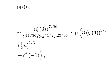
28: 26.12 Plane Partitions

… ►

26.12.2

\begin{array}[]{cccccc}6&5&5&4&3&3\\ 6&4&3&3&1\\ 6&4&3&1&1\\ 4&2&2&1\\ 3&1&1\\ 1&1&1\end{array}

ⓘ

Referenced by:: §26.12(i)
Permalink:: http://dlmf.nist.gov/26.12.E2
Encodings:: pMML, png, TeX
See also:: Annotations for §26.12(i), §26.12 and Ch.26

… ►

Table 26.12.1: Plane partitions.

► ►►►

$n$	$\operatorname{pp}\left(n\right)$	$n$	$\operatorname{pp}\left(n\right)$	$n$	$\operatorname{pp}\left(n\right)$
…
11	859	28	24 83234	45	17740 79109
…

► … ►

26.12.15

\prod_{h=0}^{r-1}\frac{(3h+1)\,(6h)!\,(2h)!}{(4h+1)!\,(4h)!}.

ⓘ

Symbols:: $!$ : factorial (as in $n!$ ), $r$ : positive integer and $h$ : positive integer
Permalink:: http://dlmf.nist.gov/26.12.E15
Encodings:: pMML, png, TeX
See also:: Annotations for §26.12(i), §26.12 and Ch.26

… ►

26.12.18

\begin{array}[]{ccccc}6&6&6&4&3\\ &3&3\\ &&2\end{array}

ⓘ

Permalink:: http://dlmf.nist.gov/26.12.E18
Encodings:: pMML, png, TeX
See also:: Annotations for §26.12(i), §26.12 and Ch.26

… ►

26.12.26

\operatorname{pp}\left(n\right)\sim\frac{\left(\zeta\left(3\right)\right)^{7/3% 6}}{2^{11/36}(3\pi)^{1/2}n^{25/36}}\exp\left(3\left(\zeta\left(3\right)\right)% ^{1/3}\left(\tfrac{1}{2}n\right)^{2/3}+\zeta'\left(-1\right)\right),

ⓘ

Symbols:: $\zeta\left(\NVar{s}\right)$ : Riemann zeta function, $\sim$ : asymptotic equality, $\exp\NVar{z}$ : exponential function, $\operatorname{pp}\left(\NVar{n}\right)$ : number of plane partitions of $n$ , $n$ : nonnegative integer and $\pi$ : plane partition
Referenced by:: §26.12(iv), Erratum (V1.0.5) for Equation (26.12.26)
Permalink:: http://dlmf.nist.gov/26.12.E26
Encodings:: pMML, png, TeX
Errata (effective with 1.0.5):: The original statement of this equation, $\operatorname{pp}\left(n\right)\sim\left(\frac{\zeta\left(3\right)}{2^{11}n^{2% 5}}\right)^{1/36}\*\exp\left(3\left(\frac{\zeta\left(3\right)n^{2}}{4}\right)^% {1/3}+\zeta'\left(-1\right)\right)$ , has been corrected.
Reported 2011-09-05 by Suresh Govindarajan
See also:: Annotations for §26.12(iv), §26.12 and Ch.26

…

29: 10.75 Tables

… ►

•

Zhang and Jin (1996, pp. 185–195) tabulates $J_{n}\left(x\right)$ , $J_{n}'\left(x\right)$ , $Y_{n}\left(x\right)$ , $Y_{n}'\left(x\right)$ , $n=0(1)10(10)50,100$ , $x=1$ , 5, 10, 25, 50, 100, 9S; $J_{n+\alpha}\left(x\right)$ , $J_{n+\alpha}'\left(x\right)$ , $Y_{n+\alpha}\left(x\right)$ , $Y_{n+\alpha}'\left(x\right)$ , $n=0(1)5,10,30,50,100$ , $\alpha=\tfrac{1}{4},\tfrac{1}{3},\tfrac{1}{2},\tfrac{2}{3},\tfrac{3}{4}$ , $x=1,5,10,50$ , 8S; real and imaginary parts of $J_{n+\alpha}\left(z\right)$ , $J_{n+\alpha}'\left(z\right)$ , $Y_{n+\alpha}\left(z\right)$ , $Y_{n+\alpha}'\left(z\right)$ , $n=0(1)15,20(10)50,100$ , $\alpha=0,\tfrac{1}{2}$ , $z=4+2i$ , $20+10i$ , 8S.

… ►

•

MacDonald (1989) tabulates the first 30 zeros, in ascending order of absolute value in the fourth quadrant, of the function $J_{0}\left(z\right)-iJ_{1}\left(z\right)$ , 6D. (Other zeros of this function can be obtained by reflection in the imaginary axis).

… ►

•

Abramowitz and Stegun (1964, Chapter 11) tabulates $\int_{0}^{x}J_{0}\left(t\right)\,\mathrm{d}t$ , $\int_{0}^{x}Y_{0}\left(t\right)\,\mathrm{d}t$ , $x=0(.1)10$ , 10D; $\int_{0}^{x}t^{-1}(1-J_{0}\left(t\right))\,\mathrm{d}t$ , $\int_{x}^{\infty}t^{-1}Y_{0}\left(t\right)\,\mathrm{d}t$ , $x=0(.1)5$ , 8D.

… ►

•

Abramowitz and Stegun (1964, Chapter 11) tabulates $e^{-x}\int_{0}^{x}I_{0}\left(t\right)\,\mathrm{d}t$ , $e^{x}\int_{x}^{\infty}K_{0}\left(t\right)\,\mathrm{d}t$ , $x=0(.1)10$ , 7D; $e^{-x}\int_{0}^{x}t^{-1}(I_{0}\left(t\right)-1)\,\mathrm{d}t$ , $xe^{x}\int_{x}^{\infty}t^{-1}K_{0}\left(t\right)\,\mathrm{d}t$ , $x=0(.1)5$ , 6D.

… ►

•

Zhang and Jin (1996, pp. 296–305) tabulates $\mathsf{j}_{n}\left(x\right)$ , $\mathsf{j}_{n}'\left(x\right)$ , $\mathsf{y}_{n}\left(x\right)$ , $\mathsf{y}_{n}'\left(x\right)$ , ${\mathsf{i}^{(1)}_{n}}\left(x\right)$ , ${\mathsf{i}^{(1)}_{n}}'\left(x\right)$ , $\mathsf{k}_{n}\left(x\right)$ , $\mathsf{k}_{n}'\left(x\right)$ , $n=0(1)10(10)30$ , 50, 100, $x=1$ , 5, 10, 25, 50, 100, 8S; $x\mathsf{j}_{n}\left(x\right)$ , $(x\mathsf{j}_{n}\left(x\right))^{\prime}$ , $x\mathsf{y}_{n}\left(x\right)$ , $(x\mathsf{y}_{n}\left(x\right))^{\prime}$ (Riccati–Bessel functions and their derivatives), $n=0(1)10(10)30$ , 50, 100, $x=1$ , 5, 10, 25, 50, 100, 8S; real and imaginary parts of $\mathsf{j}_{n}\left(z\right)$ , $\mathsf{j}_{n}'\left(z\right)$ , $\mathsf{y}_{n}\left(z\right)$ , $\mathsf{y}_{n}'\left(z\right)$ , ${\mathsf{i}^{(1)}_{n}}\left(z\right)$ , ${\mathsf{i}^{(1)}_{n}}'\left(z\right)$ , $\mathsf{k}_{n}\left(z\right)$ , $\mathsf{k}_{n}'\left(z\right)$ , $n=0(1)15$ , 20(10)50, 100, $z=4+2i$ , $20+10i$ , 8S. (For the notation replace $j, y, i, k$ by $\mathsf{j}$ , $\mathsf{y}$ , ${\mathsf{i}^{(1)}}$ , $\mathsf{k}$ , respectively.)

…

30: Bibliography L

… ►

D. Le (1985) An efficient derivative-free method for solving nonlinear equations. ACM Trans. Math. Software 11 (3), pp. 250–262.

ⓘ

Notes:: Corrigendum, ibid. 15(3) (1989), 287
External Links:: ISSN 0098-3500, Document, MathReview (T. Feagin), ZentralBlatt
Referenced by:: §3.8(iii).
Encodings:: BibTeX

… ►

A. Leitner and J. Meixner (1960) Eine Verallgemeinerung der Sphäroidfunktionen. Arch. Math. 11, pp. 29–39.

ⓘ

External Links:: ISSN 0003-9268, Document, MathReview (M. J. O. Strutt), ZentralBlatt
Referenced by:: §30.12.
Encodings:: BibTeX

… ►

H. Lotsch and M. Gray (1964) Algorithm 244: Fresnel integrals. Comm. ACM 7 (11), pp. 660–661.

ⓘ

Notes:: Includes Algol program, maximum accuracy 12D.
External Links:: ISSN 0001-0782, Document
Referenced by:: §7.25(iv).
Encodings:: BibTeX

… ►

N. A. Lukaševič (1967b) On the theory of Painlevé’s third equation. Differ. Uravn. 3 (11), pp. 1913–1923 (Russian).

ⓘ

Notes:: In Russian. English translation: Differential Equations 3(11), pp. 994–999
External Links:: MathReview (Z. Nehari), ZentralBlatt
Referenced by:: §32.10(iii), §32.8(iii), §32.9(i), §32.9(ii).
Encodings:: BibTeX

… ►

Y. L. Luke (1977a) Algorithms for rational approximations for a confluent hypergeometric function. Utilitas Math. 11, pp. 123–151.

ⓘ

External Links:: MathReview (F. Gotze), ZentralBlatt
Referenced by:: §13.31(iii).
Encodings:: BibTeX

…