applied to asymptotic expansions

SearchAdvancedHelp

(0.013 seconds)

21—30 of 66 matching pages

21: 26.8 Set Partitions: Stirling Numbers

… ►

§26.8(vi) Relations to Bernoulli Numbers

… ►

§26.8(vii) Asymptotic Approximations

… ►For asymptotic approximations for $s(n+1,k+1)$ and $S(n,k)$ that apply uniformly for $1\le k\le n$ as $n\to \mathrm{\infty }$ see Temme (1993) and Temme (2015, Chapter 34). ►For other asymptotic approximations and also expansions see Moser and Wyman (1958a) for Stirling numbers of the first kind, and Moser and Wyman (1958b), Bleick and Wang (1974) for Stirling numbers of the second kind. ►For asymptotic estimates for generalized Stirling numbers see Chelluri et al. (2000). …

22: 15.19 Methods of Computation

… ►

§15.19(i) Maclaurin Expansions

… ►For $z\in ℝ$ it is always possible to apply one of the linear transformations in §15.8(i) in such a way that the hypergeometric function is expressed in terms of hypergeometric functions with an argument in the interval $[0,\frac{1}{2}]$. … ►The relations in §15.5(ii) can be used to compute $F(a,b;c;z)$, provided that care is taken to apply these relations in a stable manner; see §3.6(ii). Initial values for moderate values of $|a|$ and $|b|$ can be obtained by the methods of §15.19(i), and for large values of $|a|$, $|b|$, or $|c|$ via the asymptotic expansions of §§15.12(ii) and 15.12(iii). ►For example, in the half-plane $\mathrm{\Re }z\le \frac{1}{2}$ we can use (15.12.2) or (15.12.3) to compute $F(a,b;c+N+1;z)$ and $F(a,b;c+N;z)$, where $N$ is a large positive integer, and then apply (15.5.18) in the backward direction. …

23: 16.5 Integral Representations and Integrals

… ►

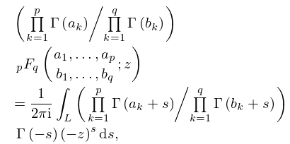
16.5.1 $$\left(\prod _{k=1}^p\mathrm{\Gamma }\left(a_k\right)/\prod _{k=1}^q\mathrm{\Gamma }\left(b_k\right)\right){}_p{}^{}F_q^{}(\genfrac{}{}{0pt}{}{a_1,\mathrm{\dots },a_p}{b_1,\mathrm{\dots },b_q};z)=\frac{1}{2\pi \mathrm{i}}{\int }_L\left(\prod _{k=1}^p\mathrm{\Gamma }\left(a_k+s\right)/\prod _{k=1}^q\mathrm{\Gamma }\left(b_k+s\right)\right)\mathrm{\Gamma }\left(-s\right){(-z)}^{s}ds,$$

ⓘ

Symbols:

$\mathrm{\Gamma }\left(z\right)$: gamma function, ${}_p{}^{}F_q^{}(a_1,\mathrm{\dots },a_p;b_1,\mathrm{\dots },b_q;z)$ or ${}_p{}^{}F_q^{}(\genfrac{}{}{0pt}{}{a_1,\mathrm{\dots },a_p}{b_1,\mathrm{\dots },b_q};z)$: alternatively ${}_p{}^{}F_q^{}(𝐚;𝐛;z)$ or ${}_p{}^{}F_q^{}(\genfrac{}{}{0pt}{}{𝐚}{𝐛};z)$
generalized hypergeometric function, $\pi$: the ratio of the circumference of a circle to its diameter, $dx$: differential of $x$ , $\mathrm{i}$: imaginary unit, $\int$: integral, $p$: nonnegative integer, $q$: nonnegative integer, $z$: complex variable, $a,a_1,\mathrm{\dots },a_p$: real or complex parameters and $b,b_1,\mathrm{\dots },b_q$: real or complex parameters

Referenced by:

§13.6(vi), §16.11(i), §16.5, §16.5

Permalink:

http://dlmf.nist.gov/16.5.E1

Encodings:

pMML, png, TeX

See also:

Annotations for §16.5 and Ch.16

… ►Suppose first that $L$ is a contour that starts at infinity on a line parallel to the positive real axis, encircles the nonnegative integers in the negative sense, and ends at infinity on another line parallel to the positive real axis. … ►Secondly, suppose that $L$ is a contour from $-\mathrm{i}\mathrm{\infty }$ to $\mathrm{i}\mathrm{\infty }$. …In the case $p=q+1$ the right-hand side of (16.5.1) supplies the analytic continuation of the left-hand side from the open unit disk to the sector ; compare §16.2(iii). …In this event, the formal power-series expansion of the left-hand side (obtained from (16.2.1)) is the asymptotic expansion of the right-hand side as $z\to 0$ in the sector $|\mathrm{ph}\left(-z\right)|\le (p+1-q-\delta )\pi /2$, where $\delta$ is an arbitrary small positive constant. …

24: 14.32 Methods of Computation

… ►Essentially the same comments that are made in §15.19 concerning the computation of hypergeometric functions apply to the functions described in the present chapter. In particular, for small or moderate values of the parameters $\mu$ and $\nu$ the power-series expansions of the various hypergeometric function representations given in §§14.3(i)–14.3(iii), 14.19(ii), and 14.20(i) can be selected in such a way that convergence is stable, and reasonably rapid, especially when the argument of the functions is real. In other cases recurrence relations (§14.10) provide a powerful method when applied in a stable direction (§3.6); see Olver and Smith (1983) and Gautschi (1967). … ►

Application of the uniform asymptotic expansions for large values of the parameters given in §§14.15 and 14.20(vii)–14.20(ix).

…

25: 11.11 Asymptotic Expansions of Anger–Weber Functions

… ►

11.11.10 $${𝐀}_{-\nu }\left(\lambda \nu \right)\sim -\frac{1}{\pi }\sum _{k=0}^{\mathrm{\infty }}\frac{(2k)!a_k(-\lambda )}{{\nu }^{2k+1}},$$ $\nu \to \mathrm{\infty }$, $|\mathrm{ph}\nu |\le \pi -\delta$.

ⓘ

Symbols:

${𝐀}_{\nu }\left(z\right)$: Anger–Weber function, $\sim$: Poincaré asymptotic expansion, $\pi$: the ratio of the circumference of a circle to its diameter, $!$: factorial (as in $n!$), $\mathrm{ph}$: phase, $\nu$: real or complex order, $k$: nonnegative integer, $\delta$: arbitrary small positive constant, $\lambda$: parameter and $a_k(\lambda )$: expansion function

Sources:

Meijer (1932); Watson (1944, §10.15); Olver (1997b, pp. 103 and 352); Nemes (2014b); Nemes (2014c)

Proof sketch:

Apply Laplace’s method to the integral (11.10.4).

Referenced by:

(11.11.18), (11.11.19), §11.11(iii), §11.11(iii)

Permalink:

http://dlmf.nist.gov/11.11.E10

Encodings:

pMML, png, TeX

Clarification (effective with 1.1.2):

The constraint which was originally $\nu \to +\mathrm{\infty }$, has been extended to be $\nu \to \mathrm{\infty }$, $|\mathrm{ph}\nu |\le \pi -\delta$.

Suggested 2021-04-05 by Gergő Nemes

See also:

Annotations for §11.11(iii), §11.11 and Ch.11

… ►

11.11.11 $${𝐀}_{-\nu }\left(\lambda \nu \right)\sim {\left(\frac{2}{\pi \nu }\right)}^{1/2}{\mathrm{e}}^{-\nu \mu }\sum _{k=0}^{\mathrm{\infty }}\frac{{\left(\frac{1}{2}\right)}_k{b}_k(\lambda )}{{\nu }^k},$$ $\nu \to \mathrm{\infty }$, $|\mathrm{ph}\nu |\le \frac{\pi }{2}-\delta$,

ⓘ

Symbols:

${\left(a\right)}_n$: Pochhammer’s symbol (or shifted factorial), ${𝐀}_{\nu }\left(z\right)$: Anger–Weber function, $\sim$: Poincaré asymptotic expansion, $\pi$: the ratio of the circumference of a circle to its diameter, $\mathrm{e}$: base of natural logarithm, $\mathrm{ph}$: phase, $\nu$: real or complex order, $k$: nonnegative integer, $\delta$: arbitrary small positive constant, $\lambda$: parameter and $b_k(\lambda )$: expansion function

Sources:

Dingle (1973, p. 388); Olver (1997b, pp. 103 and 352)

Proof sketch:

Derivable by applying Laplace’s method to the integral (11.10.4).

Permalink:

http://dlmf.nist.gov/11.11.E11

Encodings:

pMML, png, TeX

Clarification (effective with 1.1.2):

The constraint which was originally $\nu \to +\mathrm{\infty }$, has been extended to be $\nu \to \mathrm{\infty }$, $|\mathrm{ph}\nu |\le \frac{\pi }{2}-\delta$.

Suggested 2021-04-05 by Gergő Nemes

See also:

Annotations for §11.11(iii), §11.11 and Ch.11

…

26: 9.17 Methods of Computation

… ►For large $|z|$ the asymptotic expansions of §§9.7 and 9.12(viii) should be used instead. … ►But when the integration has to be towards the origin, with starting values of $\mathrm{Ai}\left(z\right)$ and ${\mathrm{Ai}}^{\prime }\left(z\right)$ computed from their asymptotic expansions. … ►The trapezoidal rule (§3.5(i)) is then applied. The second method is to apply generalized Gauss–Laguerre quadrature (§3.5(v)) to the integral (9.5.8). … ►Zeros of the Airy functions, and their derivatives, can be computed to high precision via Newton’s rule (§3.8(ii)) or Halley’s rule (§3.8(v)), using values supplied by the asymptotic expansions of §9.9(iv) as initial approximations. …

27: 8.18 Asymptotic Expansions of $I_x(a,b)$

§8.18 Asymptotic Expansions of $I_x(a,b)$

… ►

§8.18(ii) Large Parameters: Uniform Asymptotic Expansions

… ►

Symmetric Case

… ►

General Case

… ►For asymptotic expansions for large values of $a$ and/or $b$ of the $x$-solution of the equation …

28: 2.1 Definitions and Elementary Properties

… ►

§2.1(iii) Asymptotic Expansions

… ►means that for each $n$, the difference between $f(x)$ and the $n$th partial sum on the right-hand side is $O\left({(x-c)}^n\right)$ as $x\to c$ in $𝐗$. … ►

§2.1(iv) Uniform Asymptotic Expansions

… ►

§2.1(v) Generalized Asymptotic Expansions

… ►As in §2.1(iv), generalized asymptotic expansions can also have uniformity properties with respect to parameters. …

29: Bibliography N

… ►

On an asymptotic expansion of the Kontorovich-Lebedev transform. Applicable Anal. 39 (4), pp. 249–263.

ⓘ

External Links:

ISSN 0003-6811, Document, MathReview (Aloknath Chakrabarti), ZentralBlatt

Referenced by:

§10.43(v).

Encodings:

BibTeX

►

On an asymptotic expansion of the Kontorovich-Lebedev transform. Methods Appl. Anal. 3 (1), pp. 98–108.

ⓘ

External Links:

ISSN 1073-2772, FullText, MathReview (C. M. Joshi), ZentralBlatt

Referenced by:

§10.43(v).

Encodings:

BibTeX

… ►

Error bounds for the asymptotic expansion of the Hurwitz zeta function. Proc. A. 473 (2203), pp. 20170363, 16.

ⓘ

External Links:

ISSN 1364-5021, Document, Link, MathReview Entry, ZentralBlatt

Referenced by:

§8.15.

Encodings:

BibTeX

►

Uniform asymptotic expansion for the incomplete beta function. SIGMA Symmetry Integrability Geom. Methods Appl. 12, pp. 101, 5 pages.

ⓘ

External Links:

ISSN 1815-0659, Document, Link, MathReview Entry, ZentralBlatt

Referenced by:

§8.18(ii), §8.18(ii), Erratum (V1.0.14) for Subsections 8.18(ii)–8.11(v).

Encodings:

BibTeX

… ►

Error bounds and exponential improvement for Hermite’s asymptotic expansion for the gamma function. Appl. Anal. Discrete Math. 7 (1), pp. 161–179.

ⓘ

External Links:

ISSN 1452-8630, Document, FullText, MathReview (Junesang Choi), ZentralBlatt

Referenced by:

§5.11(ii), §5.11(ii).

Encodings:

BibTeX

…

30: 10.17 Asymptotic Expansions for Large Argument

§10.17 Asymptotic Expansions for Large Argument

… ►

§10.17(ii) Asymptotic Expansions of Derivatives

… ►

§10.17(iii) Error Bounds for Real Argument and Order

… ►

§10.17(v) Exponentially-Improved Expansions

… ►For higher re-expansions of the remainder terms see Olde Daalhuis and Olver (1995a) and Olde Daalhuis (1995, 1996).