§14.15 Uniform Asymptotic Approximations
Contents
- §14.15(i) Large , Fixed
- §14.15(ii) Large ,
- §14.15(iii) Large , Fixed
- §14.15(iv) Large ,
- §14.15(v) Large ,
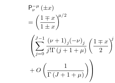
§14.15(i) Large , Fixed
For the interval with fixed , real , and arbitrary fixed values of the nonnegative integer ,
| 14.15.1 | |||
as , uniformly with respect to . In other words, the convergent hypergeometric series expansions of are also generalized (and uniform) asymptotic expansions as , with scale , ; compare §2.1(v).
Provided that the corresponding expansions for and can be obtained from the connection formulas (14.9.7), (14.9.9), and (14.9.10).
§14.15(ii) Large ,
In this and subsequent subsections denotes an arbitrary constant such that .
As ,
| 14.15.4 | |||
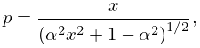
uniformly with respect to and , where
| 14.15.5 | |||
| 14.15.6 | |||
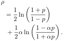
and
| 14.15.7 | |||
With the same conditions, the corresponding approximation for is obtained by replacing by on the right-hand side of (14.15.4). Approximations for and can then be achieved via (14.9.7), (14.9.9), and (14.9.10).
Next,
| 14.15.8 | |||
| 14.15.9 | |||
uniformly with respect to and . Here is again given by (14.15.5), and is defined implicitly by
| 14.15.10 | |||
The interval is mapped one-to-one to the interval , with the points and corresponding to and , respectively. For asymptotic expansions and explicit error bounds, see Dunster (2003b).
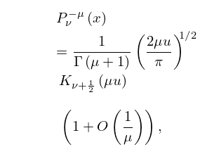
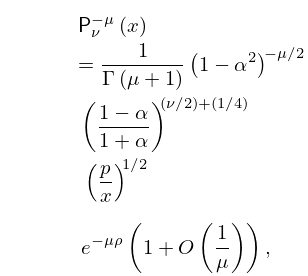
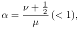
§14.15(iii) Large , Fixed
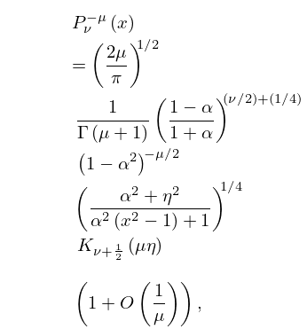
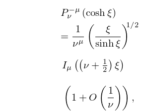
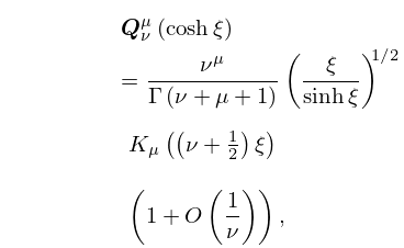
For and fixed (),
| 14.15.11 | ||||
| 14.15.12 | ||||
uniformly for . For the Bessel functions and see §10.2(ii), and for the functions associated with and see §2.8(iv).
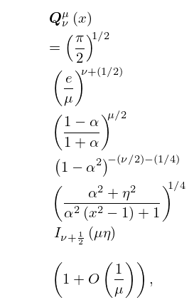
Next,
| 14.15.13 | ||||
| 14.15.14 | ||||
uniformly for .
For asymptotic expansions and explicit error bounds, see Olver (1997b, Chapter 12, §§12, 13) and Jones (2001). For convergent series expansions see Dunster (2004). See also Temme (2015, Chapter 29).
See also Olver (1997b, pp. 311–313) and §18.15(iii) for a generalized asymptotic expansion in terms of elementary functions for Legendre polynomials as with fixed.
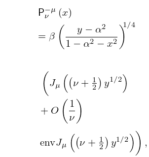
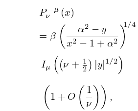
§14.15(iv) Large ,
As ,
| 14.15.15 | |||
| 14.15.16 | |||
uniformly with respect to and . For , , and see below.
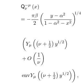
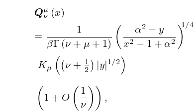
Next,
| 14.15.17 | |||
| 14.15.18 | |||
uniformly with respect to and . In (14.15.15)–(14.15.18)
| 14.15.19 | |||
| 14.15.20 | |||
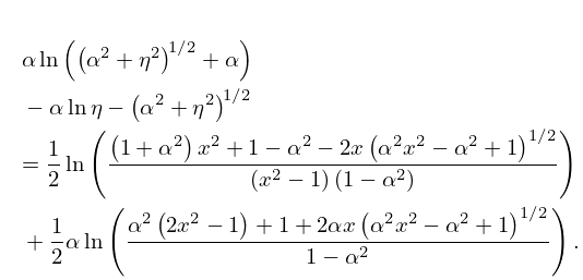
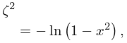
and the variable is defined implicitly by
| 14.15.21 | |||
| , , | |||
and
| 14.15.22 | |||
| , , | |||
where the inverse trigonometric functions take their principal values (§4.23(ii)). The points , , and are mapped to , , and , respectively. The interval is mapped one-to-one to the interval , where is the (positive) solution of (14.15.21) when .
For asymptotic expansions and explicit error bounds, see Boyd and Dunster (1986).
§14.15(v) Large ,
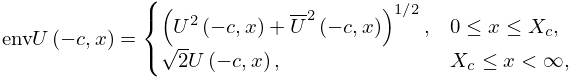
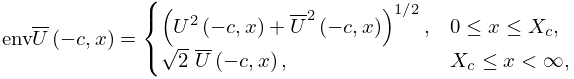
Here we introduce the envelopes of the parabolic cylinder functions , , which are defined in §12.2. For or , with and nonnegative,
| 14.15.23 | ||||
where denotes the largest positive root of the equation .
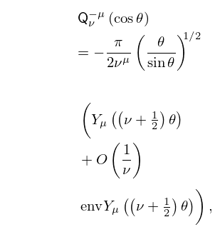
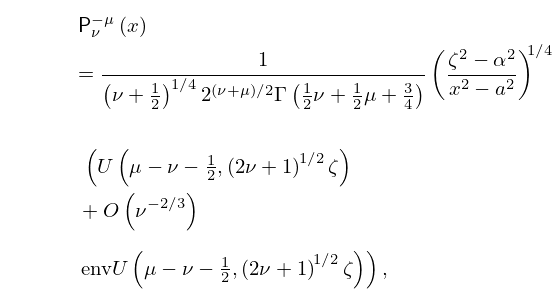
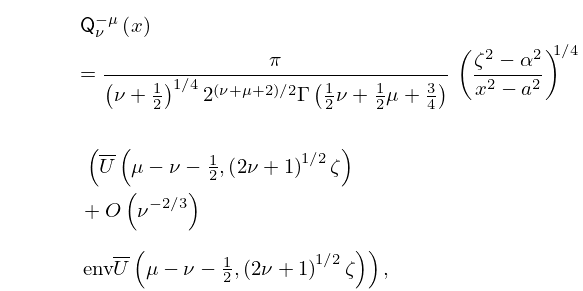
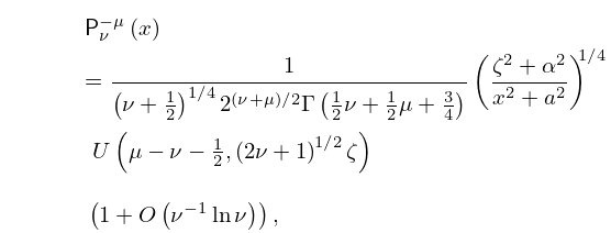
As ,
| 14.15.24 | |||
| 14.15.25 | |||
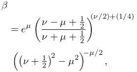
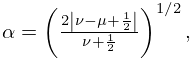
uniformly with respect to and . Here
| 14.15.26 | ||||
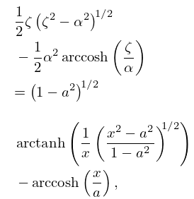
and the variable is defined implicitly by
| 14.15.27 | |||
| , , | |||
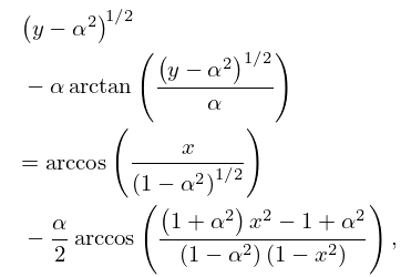
and
| 14.15.28 | |||
| , , | |||
when , and
| 14.15.29 | |||
| , | |||
when . The inverse hyperbolic and trigonometric functions take their principal values (§§4.23(ii), 4.37(ii)).
When the interval is mapped one-to-one to the interval , with the points , , and corresponding to , , and , respectively. When the interval is mapped one-to-one to the interval , with the points , , and corresponding to , , and , respectively.
Next, as ,
| 14.15.30 | |||
uniformly with respect to and . Here is defined implicitly by
| 14.15.31 | |||
| , , | |||
when , which maps the interval one-to-one to the interval : the points and correspond to and , respectively. When (14.15.29) again applies. (The inverse hyperbolic functions again take their principal values.)
Since (14.15.30) holds for negative , corresponding approximations for , uniformly valid in the interval , can be obtained from (14.9.9) and (14.9.10).
For error bounds and other extensions see Olver (1975b).
