.世界杯解说名单场次『wn4.com』风之子卡尼吉亚世界杯.w6n2c9o.2022年11月29日1时51分20秒.6cecyk0oq

SearchAdvancedHelp

(0.002 seconds)

21—30 of 178 matching pages

21: 10.75 Tables

… ►

Makinouchi (1966) tabulates all values of $j_{\nu ,m}$ and $y_{\nu ,m}$ in the interval $(0,100)$, with at least 29S. These are for $\nu =0(1)5$, 10, 20; $\nu =\frac{3}{2}$, $\frac{5}{2}$; $\nu =m/n$ with $m=1(1)n-1$ and $n=3(1)8$, except for $\nu =\frac{1}{2}$.

… ►

Abramowitz and Stegun (1964, Chapter 11) tabulates ${\int }_0^x{J}_0\left(t\right)dt$, ${\int }_0^x{Y}_0\left(t\right)dt$, $x=0(.1)10$, 10D; ${\int }_0^x{t}^{-1}(1-J_0\left(t\right))dt$, ${\int }_x^{\mathrm{\infty }}{t}^{-1}{Y}_0\left(t\right)dt$, $x=0(.1)5$, 8D.

… ►

Bickley et al. (1952) tabulates $x^{-n}{I}_n\left(x\right)$ or ${\mathrm{e}}^{-x}{I}_n\left(x\right)$, $x^n{K}_n\left(x\right)$ or ${\mathrm{e}}^x{K}_n\left(x\right)$, $n=2(1)20$, $x=0$(.01 or .1) 10(.1) 20, 8S; $I_n\left(x\right)$, $K_n\left(x\right)$, $n=0(1)20$, $x=0$ or $0.1(.1)20$, 10S.

… ►

Leung and Ghaderpanah (1979), tabulates all zeros of the principal value of $K_n\left(z\right)$, for $n=2(1)10$, 29S.

… ►

Abramowitz and Stegun (1964, Chapter 11) tabulates ${\mathrm{e}}^{-x}{\int }_0^x{I}_0\left(t\right)dt$, ${\mathrm{e}}^x{\int }_x^{\mathrm{\infty }}{K}_0\left(t\right)dt$, $x=0(.1)10$, 7D; ${\mathrm{e}}^{-x}{\int }_0^x{t}^{-1}(I_0\left(t\right)-1)dt$, $x{\mathrm{e}}^x{\int }_x^{\mathrm{\infty }}{t}^{-1}{K}_0\left(t\right)dt$, $x=0(.1)5$, 6D.

…

22: Bibliography F

… ►

Tables of Values of the Function $w(z)=e^{-z^2}(1+2i{\pi }^{-1/2}{\int }_0^z{e}^{t^2}𝑑t)$ for Complex Argument. Edited by V. A. Fok; translated from the Russian by D. G. Fry. Mathematical Tables Series, Vol. 11, Pergamon Press, Oxford.

ⓘ

External Links:

MathReview, ZentralBlatt

Referenced by:

V. N. Faddeeva and N. M. Terent’ev (1954).

Encodings:

BibTeX

… ►

Polynomial relations in the Heisenberg algebra. J. Math. Phys. 35 (11), pp. 6144–6149.

ⓘ

External Links:

ISSN 0022-2488, Document, MathReview (Shao-Ming Fei), ZentralBlatt

Referenced by:

§13.3(ii), §15.5(i), §16.3(i).

Encodings:

BibTeX

… ►

On a unified approach to transformations and elementary solutions of Painlevé equations. J. Math. Phys. 23 (11), pp. 2033–2042.

ⓘ

External Links:

ISSN 0022-2488, Document, MathReview (Hélène Airault), ZentralBlatt

Referenced by:

§32.13(i), §32.7(i), §32.7(iii).

Encodings:

BibTeX

… ►

Application of the $\tau$-function theory of Painlevé equations to random matrices: ${\mathrm{P}}_{\mathrm{VI}}$, the JUE, CyUE, cJUE and scaled limits. Nagoya Math. J. 174, pp. 29–114.

ⓘ

External Links:

ISSN 0027-7630, MathReview, ZentralBlatt

Referenced by:

§32.10(vi), §32.6(v).

Encodings:

BibTeX

… ►

Algorithm 435: Modified incomplete gamma function. Comm. ACM 15 (11), pp. 993–995.

ⓘ

Notes:

Includes Fortran code. For a Remark see ACM Trans. Math. Software 4 (1978), no. 3, pp. 296–304.

External Links:

ISSN 0001-0782, Document, Remark

Referenced by:

§8.28(ii).

Encodings:

BibTeX

…

23: 24.2 Definitions and Generating Functions

… ►

Table 24.2.5: Coefficients $b_{n,k}$ of the Bernoulli polynomials $B_n\left(x\right)={\sum }_{k=0}^n{b}_{n,k}{x}^k$.

► ►►►►►

	$k$
$n$	$0$	$1$	$2$	$3$	$4$	$5$	$6$	$7$	$8$	$9$	$10$	$11$	$12$	$13$	$14$	$15$
…
$11$	$0$	$\frac{5}{6}$	$0$	$-\frac{11}{2}$	$0$	$11$	$0$	$-11$	$0$	$\frac{55}{6}$	$-\frac{11}{2}$	$1$
$12$	$-\frac{691}{2730}$	$0$	$5$	$0$	$-\frac{33}{2}$	$0$	$22$	$0$	$-\frac{33}{2}$	$0$	$11$	$-6$	$1$
…

►

►

Table 24.2.6: Coefficients $e_{n,k}$ of the Euler polynomials $E_n\left(x\right)={\sum }_{k=0}^n{e}_{n,k}{x}^k$.

► ►►►►

	$k$
$n$	$0$	$1$	$2$	$3$	$4$	$5$	$6$	$7$	$8$	$9$	$10$	$11$	$12$	$13$	$14$	$15$
…
$11$	$\frac{691}{4}$	$0$	$-\frac{1705}{2}$	$0$	$\frac{2805}{4}$	$0$	$-231$	$0$	$\frac{165}{4}$	$0$	$-\frac{11}{2}$	$1$
…

►

24: Bibliography B

… ►

Evaluation of the incomplete gamma function of imaginary argument by Chebyshev polynomials. Math. Comp. 15 (73), pp. 7–11.

ⓘ

External Links:

FullText, MathReview (J. C. P. Miller), ZentralBlatt

Referenced by:

§8.7.

Encodings:

BibTeX

… ►

Ramanujan’s theories of elliptic functions to alternative bases. Trans. Amer. Math. Soc. 347 (11), pp. 4163–4244.

ⓘ

External Links:

ISSN 0002-9947, FullText, MathReview (J. Borwein), ZentralBlatt

Referenced by:

§15.8(v), §20.11(iii).

Encodings:

BibTeX

… ►

Vortices in Ginzburg-Landau Equations. In Proceedings of the International Congress of Mathematicians, Vol. III (Berlin, 1998), pp. 11–19.

ⓘ

External Links:

ISSN 1431-0643, FullText, MathReview Entry, ZentralBlatt

Referenced by:

§17.17.

Encodings:

BibTeX

… ►

Theoretical and experimental investigation of the elliptical annual ring antenna. IEEE Trans. Antennas and Propagation 36 (11), pp. 1526–1530.

ⓘ

External Links:

Document

Referenced by:

5th item.

Encodings:

BibTeX

… ►

Rainbow over Woolsthorpe Manor. Notes and Records Roy. Soc. London 36 (1), pp. 3–11 (1 plate).

ⓘ

External Links:

ISSN 0035-9149, Document, MathReview

Referenced by:

Sidebar 9.SB1.

Encodings:

BibTeX

…

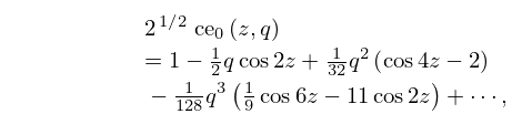
25: 28.6 Expansions for Small $q$

… ►

28.6.2 $$a_1\left(q\right)=1+q-\frac{1}{8}{q}^2-\frac{1}{64}{q}^3-\frac{1}{1536}{q}^4+\frac{11}{36864}{q}^5+\frac{49}{\mathrm{5\hspace{0.33em}89824}}{q}^6+\frac{55}{\mathrm{94\hspace{0.33em}37184}}{q}^7-\frac{83}{\mathrm{353\hspace{0.33em}89440}}{q}^8+\mathrm{\cdots },$$

ⓘ

Symbols:

$a_n\left(q\right)$: eigenvalues of Mathieu equation and $q=h^2$: parameter

Permalink:

http://dlmf.nist.gov/28.6.E2

Encodings:

pMML, png, TeX

See also:

Annotations for §28.6(i), §28.6 and Ch.28

►

28.6.3 $$b_1\left(q\right)=1-q-\frac{1}{8}{q}^2+\frac{1}{64}{q}^3-\frac{1}{1536}{q}^4-\frac{11}{36864}{q}^5+\frac{49}{\mathrm{5\hspace{0.33em}89824}}{q}^6-\frac{55}{\mathrm{94\hspace{0.33em}37184}}{q}^7-\frac{83}{\mathrm{353\hspace{0.33em}89440}}{q}^8+\mathrm{\cdots },$$

ⓘ

Symbols:

$b_n\left(q\right)$: eigenvalues of Mathieu equation and $q=h^2$: parameter

Permalink:

http://dlmf.nist.gov/28.6.E3

Encodings:

pMML, png, TeX

See also:

Annotations for §28.6(i), §28.6 and Ch.28

… ►

28.6.10 $$a_5\left(q\right)=25+\frac{1}{48}{q}^2+\frac{11}{\mathrm{7\hspace{0.33em}74144}}{q}^4+\frac{1}{\mathrm{1\hspace{0.33em}47456}}{q}^5+\frac{37}{\mathrm{8918\hspace{0.33em}13888}}{q}^6+\mathrm{\cdots },$$

ⓘ

Symbols:

$a_n\left(q\right)$: eigenvalues of Mathieu equation and $q=h^2$: parameter

Permalink:

http://dlmf.nist.gov/28.6.E10

Encodings:

pMML, png, TeX

See also:

Annotations for §28.6(i), §28.6 and Ch.28

►

28.6.11 $$b_5\left(q\right)=25+\frac{1}{48}{q}^2+\frac{11}{\mathrm{7\hspace{0.33em}74144}}{q}^4-\frac{1}{\mathrm{1\hspace{0.33em}47456}}{q}^5+\frac{37}{\mathrm{8918\hspace{0.33em}13888}}{q}^6+\mathrm{\cdots },$$

ⓘ

Symbols:

$b_n\left(q\right)$: eigenvalues of Mathieu equation and $q=h^2$: parameter

Permalink:

http://dlmf.nist.gov/28.6.E11

Encodings:

pMML, png, TeX

See also:

Annotations for §28.6(i), §28.6 and Ch.28

… ►

28.6.21 $$2^{1/2}{\mathrm{ce}}_0(z,q)=1-\frac{1}{2}q\cos 2z+\frac{1}{32}{q}^2\left(\cos 4z-2\right)-\frac{1}{128}{q}^3\left(\frac{1}{9}\cos 6z-11\cos 2z\right)+\mathrm{\cdots },$$

ⓘ

Symbols:

${\mathrm{ce}}_n(z,q)$: Mathieu function, $\cos z$: cosine function, $q=h^2$: parameter and $z$: complex variable

A&S Ref:

20.2.27

Referenced by:

§28.6(ii)

Permalink:

http://dlmf.nist.gov/28.6.E21

Encodings:

pMML, png, TeX

See also:

Annotations for §28.6(ii), §28.6 and Ch.28

…

26: 8.26 Tables

… ►

Khamis (1965) tabulates $P(a,x)$ for $a=0.05(.05)10(.1)20(.25)70$, $0.0001\le x\le 250$ to 10D.

… ►

Pearson (1968) tabulates $I_x(a,b)$ for $x=0.01(.01)1$, $a,b=0.5(.5)11(1)50$, with $b\le a$, to 7D.

… ►

Abramowitz and Stegun (1964, pp. 245–248) tabulates $E_n\left(x\right)$ for $n=2,3,4,10,20$, $x=0(.01)2$ to 7D; also $(x+n){\mathrm{e}}^x{E}_n\left(x\right)$ for $n=2,3,4,10,20$, $x^{-1}=0(.01)0.1(.05)0.5$ to 6S.

… ►

Pagurova (1961) tabulates $E_n\left(x\right)$ for $n=0(1)20$, $x=0(.01)2(.1)10$ to 4-9S; ${\mathrm{e}}^x{E}_n\left(x\right)$ for $n=2(1)10$, $x=10(.1)20$ to 7D; ${\mathrm{e}}^x{E}_p\left(x\right)$ for $p=0(.1)1$, $x=0.01(.01)7(.05)12(.1)20$ to 7S or 7D.

… ►

Zhang and Jin (1996, Table 19.1) tabulates $E_n\left(x\right)$ for $n=1,2,3,5,10,15,20$, $x=0(.1)1,1.5,2,3,5,10,20,30,50,100$ to 7D or 8S.

27: 7.23 Tables

… ►

Abramowitz and Stegun (1964, Chapter 7) includes $\mathrm{erf}x$, $(2/\sqrt{\pi }){\mathrm{e}}^{-x^2}$, $x\in [0,2]$, 10D; $(2/\sqrt{\pi }){\mathrm{e}}^{-x^2}$, $x\in [2,10]$, 8S; $x{\mathrm{e}}^{x^2}\mathrm{erfc}x$, $x^{-2}\in [0,0.25]$, 7D; $2^n\mathrm{\Gamma }\left(\frac{1}{2}n+1\right){\mathrm{i}}^n\mathrm{erfc}\left(x\right)$, $n=1(1)6,10,11$, $x\in [0,5]$, 6S; $F\left(x\right)$, $x\in [0,2]$, 10D; $xF\left(x\right)$, $x^{-2}\in [0,0.25]$, 9D; $C\left(x\right)$, $S\left(x\right)$, $x\in [0,5]$, 7D; $\mathrm{f}\left(x\right)$, $\mathrm{g}\left(x\right)$, $x\in [0,1]$, $x^{-1}\in [0,1]$, 15D.

… ►

Zhang and Jin (1996, pp. 638, 640–641) includes the real and imaginary parts of $\mathrm{erf}z$, $x\in [0,5]$, $y=0.5(.5)3$, 7D and 8D, respectively; the real and imaginary parts of ${\int }_x^{\mathrm{\infty }}{\mathrm{e}}^{\pm \mathrm{i}{t}^2}dt$, $(1/\sqrt{\pi }){\mathrm{e}}^{\mp \mathrm{i}(x^2+(\pi /4))}{\int }_x^{\mathrm{\infty }}{\mathrm{e}}^{\pm \mathrm{i}{t}^2}dt$, $x=0(.5)20(1)25$, 8D, together with the corresponding modulus and phase to 8D and 6D (degrees), respectively.

… ►

Fettis et al. (1973) gives the first 100 zeros of $\mathrm{erf}z$ and $w\left(z\right)$ (the table on page 406 of this reference is for $w\left(z\right)$, not for $\mathrm{erfc}z$), 11S.

…

28: Bibliography W

… ►

The Nahm equations, finite-gap potentials and Lamé functions. J. Phys. A 20 (10), pp. 2679–2683.

ⓘ

External Links:

ISSN 0305-4470, Document, MathReview (James M. D’Archangelo), ZentralBlatt

Referenced by:

§29.19(ii).

Encodings:

BibTeX

… ►

Rapid approximation to the Voigt/Faddeeva function and its derivatives. J. Quant. Spect. and Rad. Transfer 62 (1), pp. 29–48.

ⓘ

Notes:

Includes Fortran code in the appendices to compute the functions to an accuracy between ${10}^{-2}$ and ${10}^{-5}$.

External Links:

ISSN 0022-4073, Document

Referenced by:

§7.21, §7.21.

Encodings:

BibTeX

… ►

Some hypergeometric orthogonal polynomials. SIAM J. Math. Anal. 11 (4), pp. 690–701.

ⓘ

External Links:

ISSN 0036-1410, Document, MathReview (R. G. Buschman), ZentralBlatt

Referenced by:

§18.25(i), §18.25(i), §18.25(ii), §18.25(iii), §18.26(i), §18.26(ii), §18.38(iii).

Encodings:

BibTeX

… ►

On the asymptotic behavior of the Fourier coefficients of Mathieu functions. J. Res. Nat. Inst. Standards Tech. 113 (1), pp. 11–15.

ⓘ

External Links:

ISSN 1044-677X, FullText

Referenced by:

§28.4(vii).

Encodings:

BibTeX

… ►

The generalized Bessel function of order greater than one. Quart. J. Math., Oxford Ser. 11, pp. 36–48.

ⓘ

External Links:

Document, MathReview (M. C. Gray), ZentralBlatt

Referenced by:

§10.46.

Encodings:

BibTeX

…

29: 6.19 Tables

… ►

Abramowitz and Stegun (1964, Chapter 5) includes $x^{-1}\mathrm{Si}\left(x\right)$, $-x^{-2}\mathrm{Cin}\left(x\right)$, $x^{-1}\mathrm{Ein}\left(x\right)$, $-x^{-1}\mathrm{Ein}\left(-x\right)$, $x=0(.01)0.5$; $\mathrm{Si}\left(x\right)$, $\mathrm{Ci}\left(x\right)$, $\mathrm{Ei}\left(x\right)$, $E_1\left(x\right)$, $x=0.5(.01)2$; $\mathrm{Si}\left(x\right)$, $\mathrm{Ci}\left(x\right)$, $x{\mathrm{e}}^{-x}\mathrm{Ei}\left(x\right)$, $x{\mathrm{e}}^x{E}_1\left(x\right)$, $x=2(.1)10$; $x\mathrm{f}\left(x\right)$, $x^2\mathrm{g}\left(x\right)$, $x{\mathrm{e}}^{-x}\mathrm{Ei}\left(x\right)$, $x{\mathrm{e}}^x{E}_1\left(x\right)$, $x^{-1}=0(.005)0.1$; $\mathrm{Si}\left(\pi x\right)$, $\mathrm{Cin}\left(\pi x\right)$, $x=0(.1)10$. Accuracy varies but is within the range 8S–11S.

►

Zhang and Jin (1996, pp. 652, 689) includes $\mathrm{Si}\left(x\right)$, $\mathrm{Ci}\left(x\right)$, $x=0(.5)20(2)30$, 8D; $\mathrm{Ei}\left(x\right)$, $E_1\left(x\right)$, $x=[0,100]$, 8S.

… ►

Abramowitz and Stegun (1964, Chapter 5) includes the real and imaginary parts of $z{\mathrm{e}}^z{E}_1\left(z\right)$, $x=-19(1)20$, $y=0(1)20$, 6D; ${\mathrm{e}}^z{E}_1\left(z\right)$, $x=-4(.5)-2$, $y=0(.2)1$, 6D; $E_1\left(z\right)+\ln z$, $x=-2(.5)2.5$, $y=0(.2)1$, 6D.

►

Zhang and Jin (1996, pp. 690–692) includes the real and imaginary parts of $E_1\left(z\right)$, $\pm x=0.5,1,3,5,10,15,20,50,100$, $y=0(.5)1(1)5(5)30,50,100$, 8S.

30: Bibliography S

… ►

On integral representations for Lamé and other special functions. SIAM J. Math. Anal. 11 (4), pp. 702–723.

ⓘ

External Links:

ISSN 0036-1410, Document, MathReview (R. K. Gupta), ZentralBlatt

Referenced by:

§29.17(i), §29.8.

Encodings:

BibTeX

… ►

The Laplace transforms of products of Airy functions. Dirāsāt Ser. B Pure Appl. Sci. 19 (2), pp. 7–11.

ⓘ

External Links:

ISSN 0253-424X, MathReview

Referenced by:

§9.10(v).

Encodings:

BibTeX

… ►

A simple approach to asymptotic expansions for Fourier integrals of singular functions. Appl. Math. Comput. 216 (11), pp. 3378–3385.

ⓘ

External Links:

ISSN 0096-3003, Document, Link, MathReview Entry, ZentralBlatt

Referenced by:

§2.3(iv).

Encodings:

BibTeX

… ►

Représentation asymptotique de la solution générale de l’équation de Mathieu-Hill. Acad. Roy. Belg. Bull. Cl. Sci. (5) 51 (11), pp. 1415–1446.

ⓘ

External Links:

ZentralBlatt

Referenced by:

§28.8(ii).

Encodings:

BibTeX

… ►

Exact error terms in the asymptotic expansion of a class of integral transforms. I. Oscillatory kernels. SIAM J. Math. Anal. 11 (5), pp. 828–841.

ⓘ

External Links:

ISSN 0036-1410, Document, MathReview (John S. Lew), ZentralBlatt

Referenced by:

§2.5(ii).

Encodings:

BibTeX

…