.樊振东世界杯冠军_『wn4.com_』cntv能否看世界杯_w6n2c9o_2022年11月29日22时14分2秒_2kukma4ks_gov_hk
(0.004 seconds)
21—30 of 848 matching pages
21: 24.19 Methods of Computation
…
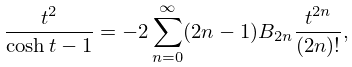
►If denotes the right-hand side of (24.19.1) but with the second product taken only for , then for .
…
►For other information see Chellali (1988) and Zhang and Jin (1996, pp. 1–11).
For algorithms for computing , , , and see Spanier and Oldham (1987, pp. 37, 41, 171, and 179–180).
…
►For number-theoretic applications it is important to compute for ; in particular to find the irregular pairs
for which .
…
►
•
…
22: Bibliography E
…
►
The penetration of a potential barrier by electrons.
Phys. Rev. 35 (11), pp. 1303–1309.
…
►
Painlevé transcendent describes quantum correlation function of the antiferromagnet away from the free-fermion point.
J. Phys. A 29 (17), pp. 5619–5626.
…
►
Institutiones Calculi Integralis.
Opera Omnia (1), Vol. 11, pp. 110–113.
…
►
The Sobolev orthogonality and spectral analysis of the Laguerre polynomials for positive integers
.
J. Comput. Appl. Math. 171 (1-2), pp. 199–234.
…
►
Note on the -Laguerre orthogonal polynomials.
…
23: Bibliography K
…
►
Auxiliary table for the incomplete elliptic integrals.
J. Math. Physics 27, pp. 11–36.
…
►
The asymptotic expansion of a hypergeometric function
.
Math. Comp. 26 (120), pp. 963.
…
►
An extension of Saalschütz’s summation theorem for the series
.
Integral Transforms Spec. Funct. 24 (11), pp. 916–921.
…
►
Algorithm 327: Dilogarithm [S22].
Comm. ACM 11 (4), pp. 270–271.
…
►
Clebsch-Gordan coefficients for and Hahn polynomials.
Nieuw Arch. Wisk. (3) 29 (2), pp. 140–155.
…
24: Bibliography L
…
►
Eine Verallgemeinerung der Sphäroidfunktionen.
Arch. Math. 11, pp. 29–39.
…
►
Note sur la fonction
.
Acta Math. 11 (1-4), pp. 19–24 (French).
…
►
Algorithm 244: Fresnel integrals.
Comm. ACM 7 (11), pp. 660–661.
…
►
On the theory of Painlevé’s third equation.
Differ. Uravn. 3 (11), pp. 1913–1923 (Russian).
…
►
Algorithms for rational approximations for a confluent hypergeometric function.
Utilitas Math. 11, pp. 123–151.
…
25: Bibliography H
…
►
La -conjecture de Macdonald-Morris pour
.
C. R. Acad. Sci. Paris Sér. I Math. 303 (6), pp. 211–213 (French).
…
►
25D Table of the First One Hundred Values of ,, ,,,
.
Technical report
Department of Physics, Worcester Polytechnic Institute, Worcester, MA.
…
►
Inverse virial symmetry of diatomic potential curves.
J. Chem. Phys. 109 (1), pp. 11–19.
…
►
Algorithm 395: Student’s t-distribution.
Comm. ACM 13 (10), pp. 617–619.
►
Algorithm 571: Statistics for von Mises’ and Fisher’s distributions of directions: , and their inverses [S14].
ACM Trans. Math. Software 7 (2), pp. 233–238.
…
26: Bibliography O
…
►
Studies on the Painlevé equations. III. Second and fourth Painlevé equations, and
.
Math. Ann. 275 (2), pp. 221–255.
…
►
Triorthogonal systems in spaces of constant curvature in which the equation allows a complete separation of variables.
Mat. Sbornik N.S. 27(69) (3), pp. 379–426 (Russian).
…
►
Error bounds for stationary phase approximations.
SIAM J. Math. Anal. 5 (1), pp. 19–29.
…
►
Numerical solution of Riemann-Hilbert problems: Painlevé II.
Found. Comput. Math. 11 (2), pp. 153–179.
…
►
Algorithm 22: Riccati-Bessel functions of first and second kind.
Comm. ACM 3 (11), pp. 600–601.
…
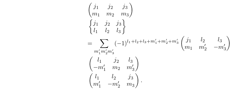
27: 34.5 Basic Properties: Symbol
…
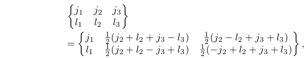
►If any lower argument in a symbol is , , or , then the symbol has a simple algebraic form.
…
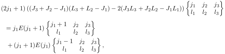
►
34.5.9
…
►
34.5.11
…
►
34.5.16
…
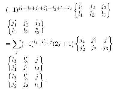
►
34.5.23
…
28: Bibliography D
…
►
Real zeros of hypergeometric polynomials.
J. Comput. Appl. Math. 247, pp. 152–161.
…
►
Algorithm 322. F-distribution.
Comm. ACM 11 (2), pp. 116–117.
…
►
Theta functions and non-linear equations.
Uspekhi Mat. Nauk 36 (2(218)), pp. 11–80 (Russian).
…
►
Uniform asymptotic approximations for the Whittaker functions and
.
Anal. Appl. (Singap.) 1 (2), pp. 199–212.
…
►
The incomplete beta function—a historical profile.
Arch. Hist. Exact Sci. 24 (1), pp. 11–29.
…
29: 11.14 Tables
…
►
•
…
►
•
►
•
…
►
•
…
►
•
Abramowitz and Stegun (1964, Chapter 12) tabulates , , and for and , to 6D or 7D.
Abramowitz and Stegun (1964, Chapter 12) tabulates and for to 5D or 7D; , , and for to 6D.
Agrest et al. (1982) tabulates and for to 11D.
Jahnke and Emde (1945) tabulates for and to 4D.
Agrest and Maksimov (1971, Chapter 11) defines incomplete Struve, Anger, and Weber functions and includes tables of an incomplete Struve function for , , and , together with surface plots.
