differential%20equation

(0.002 seconds)

11—20 of 28 matching pages

11: 3.8 Nonlinear Equations

… ►The equation to be solved is … ►This is useful when

f(z)

satisfies a second-order linear differential equation because of the ease of computing

f^{\prime\prime}(z_{n})

. … ►For describing the distribution of complex zeros of solutions of linear homogeneous second-order differential equations by methods based on the Liouville–Green (WKB) approximation, see Segura (2013). … ►Consider

x=20

and

j=19

. We have

p^{\mspace{1.0mu}\prime}(20)=19!

and

a_{19}=1+2+\dots+20=210

. …

12: Bibliography M

… ►

A. P. Magnus (1995) Painlevé-type differential equations for the recurrence coefficients of semi-classical orthogonal polynomials. J. Comput. Appl. Math. 57 (1-2), pp. 215–237.

ⓘ

External Links:: ISSN 0377-0427, Document, MathReview (Leonid B. Golinskiĭ), ZentralBlatt
Referenced by:: §32.15.
Encodings:: BibTeX

… ►

W. Magnus and S. Winkler (1966) Hill’s Equation. Interscience Tracts in Pure and Applied Mathematics, No. 20, Interscience Publishers John Wiley & Sons, New York-London-Sydney.

ⓘ

Notes:: Reprinted by Dover Publications, Inc., New York, 1979.
External Links:: MathReview (H. Hochstadt), ZentralBlatt
Referenced by:: §1.3(iii), §28.29(i), §28.29(ii), §28.29(ii), §28.29(iii), §28.29(iii), §28.29(iii), §28.30(i), Ch.28, §29.3(i), §29.9.
Encodings:: BibTeX

… ►

R. S. Maier (2005) On reducing the Heun equation to the hypergeometric equation. J. Differential Equations 213 (1), pp. 171–203.

ⓘ

External Links:: ISSN 0022-0396, Document, MathReview (Wolfgang Bühring), ZentralBlatt
Referenced by:: §31.7(i).
Encodings:: BibTeX

… ►

J. C. P. Miller (1950) On the choice of standard solutions for a homogeneous linear differential equation of the second order. Quart. J. Mech. Appl. Math. 3 (2), pp. 225–235.

ⓘ

External Links:: Document, MathReview (W. R. Wasow), ZentralBlatt
Referenced by:: §12.2(vi), §2.7(iv), §2.7(iv).
Encodings:: BibTeX

… ►

K. S. Miller and B. Ross (1993) An Introduction to the Fractional Calculus and Fractional Differential Equations. A Wiley-Interscience Publication, John Wiley & Sons, Inc., New York.

ⓘ

External Links:: ISBN 0-471-58884-9, MathReview (K. C. Gupta), ZentralBlatt
Referenced by:: §1.15(vi), Erratum (V1.0.14) for Subsections 1.15(vi), 1.15(vii), 2.6(iii).
Encodings:: BibTeX

…

13: Bibliography O

… ►

A. B. Olde Daalhuis and F. W. J. Olver (1995a) Hyperasymptotic solutions of second-order linear differential equations. I. Methods Appl. Anal. 2 (2), pp. 173–197.

ⓘ

External Links:: ISSN 1073-2772, FullText, MathReview (A. D. Wood), ZentralBlatt
Referenced by:: §10.17(v), §10.40(iv), §13.29(i), §13.7(iii), §2.11(v), §9.7(v).
Encodings:: BibTeX

►

A. B. Olde Daalhuis and F. W. J. Olver (1995b) On the calculation of Stokes multipliers for linear differential equations of the second order. Methods Appl. Anal. 2 (3), pp. 348–367.

ⓘ

External Links:: ISSN 1073-2772, Pdf, MathReview (Archibald D. MacGillivray), ZentralBlatt
Referenced by:: §2.7(ii).
Encodings:: BibTeX

►

A. B. Olde Daalhuis and F. W. J. Olver (1998) On the asymptotic and numerical solution of linear ordinary differential equations. SIAM Rev. 40 (3), pp. 463–495.

ⓘ

External Links:: ISSN 1095-7200, Document, MathReview (W. Balser), ZentralBlatt
Referenced by:: §16.25, §2.7(ii), §3.7(iii).
Encodings:: BibTeX

… ►

F. W. J. Olver (1977c) Second-order differential equations with fractional transition points. Trans. Amer. Math. Soc. 226, pp. 227–241.

ⓘ

External Links:: FullText, MathReview (Anthony Leung), ZentralBlatt
Referenced by:: §2.8(v).
Encodings:: BibTeX

… ►

P. J. Olver (1993b) Applications of Lie Groups to Differential Equations. 2nd edition, Graduate Texts in Mathematics, Vol. 107, Springer-Verlag, New York.

ⓘ

External Links:: ISBN 0-387-94007-3; 0-387-95000-1, MathReview, ZentralBlatt
Referenced by:: §32.13(i).
Encodings:: BibTeX

…

14: Bibliography I

… ►

E. L. Ince (1926) Ordinary Differential Equations. Longmans, Green and Co., London.

ⓘ

Notes:: Reprinted by Dover Publications, New York, 1944, 1956.
External Links:: MathReview, ZentralBlatt
Referenced by:: §1.13(i), §1.13(i), §1.13(i), §31.12, §31.14(i), §32.2(i), §32.2(vi), Erratum (V1.0.25) for Section 1.13.
Encodings:: BibTeX

… ►

K. Inkeri (1959) The real roots of Bernoulli polynomials. Ann. Univ. Turku. Ser. A I 37, pp. 1–20.

ⓘ

External Links:: MathReview (D. H. Lehmer), ZentralBlatt
Referenced by:: §24.12(i).
Encodings:: BibTeX

… ►

A. Iserles (1996) A First Course in the Numerical Analysis of Differential Equations. Cambridge Texts in Applied Mathematics, No. 15, Cambridge University Press, Cambridge.

ⓘ

External Links:: ISBN 0-521-55376-8; 0-521-55655-4, MathReview (Luis Verde-Star), ZentralBlatt
Referenced by:: §3.7(i).
Encodings:: BibTeX

… ►

A. R. Its, A. S. Fokas, and A. A. Kapaev (1994) On the asymptotic analysis of the Painlevé equations via the isomonodromy method. Nonlinearity 7 (5), pp. 1291–1325.

ⓘ

External Links:: ISSN 0951-7715, Document, MathReview (Alexander Vladimirovich Kitaev), ZentralBlatt
Referenced by:: §32.11(iii).
Encodings:: BibTeX

… ►

A. R. Its and V. Yu. Novokshënov (1986) The Isomonodromic Deformation Method in the Theory of Painlevé Equations. Lecture Notes in Mathematics, Vol. 1191, Springer-Verlag, Berlin.

ⓘ

External Links:: ISBN 3-540-16483-9, MathReview (Alexander A. Pankov), ZentralBlatt
Referenced by:: §32.11(iv), §32.4(i), Profile Alexander A. Its.
Encodings:: BibTeX

…

15: 30.9 Asymptotic Approximations and Expansions

§30.9 Asymptotic Approximations and Expansions

… ►

30.9.1

\lambda^{m}_{n}\left(\gamma^{2}\right)\sim-\gamma^{2}+\gamma q+\beta_{0}+\beta% _{1}\gamma^{-1}+\beta_{2}\gamma^{-2}+\cdots,

ⓘ

Symbols:: $\sim$ : Poincaré asymptotic expansion, $\lambda^{\NVar{m}}_{\NVar{n}}\left(\NVar{\gamma^{2}}\right)$ : eigenvalues of the spheroidal differential equation, $m$ : nonnegative integer, $n\geq m$ : integer degree, $\gamma^{2}$ : real parameter, $q$ and $\beta_{n}$ : coeffients
A&S Ref:: 21.7.6
Referenced by:: item
Permalink:: http://dlmf.nist.gov/30.9.E1
Encodings:: pMML, png, TeX
See also:: Annotations for §30.9(i), §30.9 and Ch.30

… ►

2^{20}\beta_{5}=-527q^{7}-61529q^{5}-10\;43961q^{3}-22\;41599q+32m^{2}(5739q^{% 5}+1\;27550q^{3}+2\;98951q)-2048m^{4}(355q^{3}+1505q)+65536m^{6}q.

… ►

30.9.4

\lambda^{m}_{n}\left(\gamma^{2}\right)\sim 2q|\gamma|+c_{0}+c_{1}|\gamma|^{-1}% +c_{2}|\gamma|^{-2}+\cdots,

ⓘ

Symbols:: $\sim$ : Poincaré asymptotic expansion, $\lambda^{\NVar{m}}_{\NVar{n}}\left(\NVar{\gamma^{2}}\right)$ : eigenvalues of the spheroidal differential equation, $m$ : nonnegative integer, $n\geq m$ : integer degree, $\gamma^{2}$ : real parameter, $q$ and $c_{n}$ : coeffients
A&S Ref:: 21.8.2
Referenced by:: item
Permalink:: http://dlmf.nist.gov/30.9.E4
Encodings:: pMML, png, TeX
See also:: Annotations for §30.9(ii), §30.9 and Ch.30

… ►

16: Errata

… ►

Equation (2.3.6)

2.3.6

\mathcal{V}_{a,b}\left(f(t)\right)=\int_{a}^{b}\left|f^{\prime}(t)\right|\,% \mathrm{d}t

The integrand has been corrected so that the absolute value does not include the differential.

Reported by Juan Luis Varona on 2021-02-08

… ►

Equation (1.4.34)

1.4.34

\mathcal{V}_{a,b}\left(f\right)=\int^{b}_{a}\left|f^{\prime}(x)\right|\,% \mathrm{d}x

The integrand has been corrected so that the absolute value does not include the differential.

Reported by Tran Quoc Viet on 2020-08-11

… ►

Equations (10.15.1), (10.38.1)

These equations have been generalized to include the additional cases of $\ifrac{\partial J_{-\nu}\left(z\right)}{\partial\nu}$ , $\ifrac{\partial I_{-\nu}\left(z\right)}{\partial\nu}$ , respectively.

… ►

Chapters 8, 20, 36

Several new equations have been added. See (8.17.24), (20.7.34), §20.11(v), (26.12.27), (36.2.28), and (36.2.29).

… ►

Equation (22.16.14)

22.16.14

\mathcal{E}\left(x,k\right)=\int_{0}^{\operatorname{sn}\left(x,k\right)}\sqrt{% \frac{1-k^{2}t^{2}}{1-t^{2}}}\,\mathrm{d}t

Originally this equation appeared with the upper limit of integration as $x$ , rather than $\operatorname{sn}\left(x,k\right)$ .

Reported 2010-07-08 by Charles Karney.

…

17: 18.40 Methods of Computation

… ►Usually, however, other methods are more efficient, especially the numerical solution of difference equations (§3.6) and the application of uniform asymptotic expansions (when available) for OP’s of large degree. … … ►In what follows we consider only the simple, illustrative, case that

\mu(x)

is continuously differentiable so that

\,\mathrm{d}\mu(x)=w(x)\,\mathrm{d}x

, with

w(x)

real, positive, and continuous on a real interval

[a,b].

The strategy will be to: 1) use the moments to determine the recursion coefficients

\alpha_{n},\beta_{n}

of equations (18.2.11_5) and (18.2.11_8); then, 2) to construct the quadrature abscissas

x_{i}

and weights (or Christoffel numbers)

w_{i}

from the J-matrix of §3.5(vi), equations (3.5.31) and(3.5.32). … ►Results of low (

~{}2

3

decimal digits) precision for

w(x)

are easily obtained for

N\sim 10

20

. … ►Equation (18.40.7) provides step-histogram approximations to

\int_{a}^{x}\,\mathrm{d}\mu(x)

, as shown in Figure 18.40.1 for

N=12

and

120

, shown here for the repulsive Coulomb–Pollaczek OP’s of Figure 18.39.2, with the parameters as listed therein. …

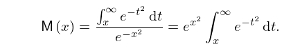
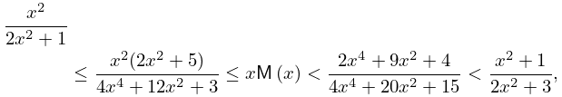
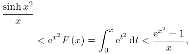
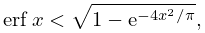
18: 7.8 Inequalities

… ►

7.8.1

\mathsf{M}\left(x\right)=\frac{\int_{x}^{\infty}e^{-t^{2}}\,\mathrm{d}t}{e^{-x% ^{2}}}=e^{x^{2}}\int_{x}^{\infty}e^{-t^{2}}\,\mathrm{d}t.

ⓘ

Defines:: $\mathsf{M}\left(\NVar{x}\right)$ : Mills’ ratio
Symbols:: $\,\mathrm{d}\NVar{x}$ : differential of $x$ , $\mathrm{e}$ : base of natural logarithm, $\int$ : integral and $x$ : real variable
Permalink:: http://dlmf.nist.gov/7.8.E1
Encodings:: pMML, png, TeX
See also:: Annotations for §7.8 and Ch.7

… ►

7.8.5

\frac{x^{2}}{2x^{2}+1}\leq\frac{x^{2}(2x^{2}+5)}{4x^{4}+12x^{2}+3}\leq x% \mathsf{M}\left(x\right)<\frac{2x^{4}+9x^{2}+4}{4x^{4}+20x^{2}+15}<\frac{x^{2}% +1}{2x^{2}+3},

x\geq 0

ⓘ

Symbols:: $\mathsf{M}\left(\NVar{x}\right)$ : Mills’ ratio and $x$ : real variable
Referenced by:: §7.8
Permalink:: http://dlmf.nist.gov/7.8.E5
Encodings:: pMML, png, TeX
See also:: Annotations for §7.8 and Ch.7

… ►

7.8.6

\int_{0}^{x}e^{at^{2}}\,\mathrm{d}t<\frac{1}{3ax}\left(2e^{ax^{2}}+ax^{2}-2% \right),

a,x>0

ⓘ

Symbols:: $\,\mathrm{d}\NVar{x}$ : differential of $x$ , $\mathrm{e}$ : base of natural logarithm, $\int$ : integral and $x$ : real variable
Referenced by:: §7.8
Permalink:: http://dlmf.nist.gov/7.8.E6
Encodings:: pMML, png, TeX
See also:: Annotations for §7.8 and Ch.7

►

7.8.7

\frac{\sinh x^{2}}{x}<{\mathrm{e}}^{x^{2}}F\left(x\right)=\int_{0}^{x}{\mathrm% {e}}^{t^{2}}\,\mathrm{d}t<\frac{{\mathrm{e}}^{x^{2}}-1}{x},

x>0

ⓘ

Symbols:: $F\left(\NVar{z}\right)$ : Dawson’s integral, $\,\mathrm{d}\NVar{x}$ : differential of $x$ , $\mathrm{e}$ : base of natural logarithm, $\sinh\NVar{z}$ : hyperbolic sine function, $\int$ : integral and $x$ : real variable
Referenced by:: Erratum (V1.1.5) for Additions
Permalink:: http://dlmf.nist.gov/7.8.E7
Encodings:: pMML, png, TeX
Addition (effective with 1.1.5):: A new inequality was added.
See also:: Annotations for §7.8 and Ch.7

… ►

7.8.8

\operatorname{erf}x<\sqrt{1-{\mathrm{e}}^{-4x^{2}/\pi}},

x>0

ⓘ

Symbols:: $\pi$ : the ratio of the circumference of a circle to its diameter, $\operatorname{erf}\NVar{z}$ : error function, $\mathrm{e}$ : base of natural logarithm and $x$ : real variable
Source:: Pólya (1949, (1.5))
Referenced by:: §7.8, Erratum (V1.0.17) for Equation (7.8.8)
Permalink:: http://dlmf.nist.gov/7.8.E8
Encodings:: pMML, png, TeX
Addition (effective with 1.0.17):: This inequality was added. It is Pólya (1949, (1.5)). Note that it is a special case of (8.10.11).
Suggested by Roberto Iacono
See also:: Annotations for §7.8 and Ch.7

19: 12.10 Uniform Asymptotic Expansions for Large Parameter

… ►

12.10.33

\mathsf{A}_{s+1}(\tau)=-4\tau^{2}(\tau+1)^{2}\frac{\mathrm{d}}{\mathrm{d}\tau}% \mathsf{A}_{s}(\tau)-\frac{1}{4}\int_{0}^{\tau}\left(20u^{2}+20u+3\right)% \mathsf{A}_{s}(u)\,\mathrm{d}u,

s=0,1,2,\dots

ⓘ

Defines:: $\mathsf{A}_{s}(\tau)$ : coefficients (locally)
Symbols:: $\frac{\mathrm{d}\NVar{f}}{\mathrm{d}\NVar{x}}$ : derivative of $f$ with respect to $x$ , $\,\mathrm{d}\NVar{x}$ : differential of $x$ , $\int$ : integral, $s$ : nonnegative integer and $\tau$
Permalink:: http://dlmf.nist.gov/12.10.E33
Encodings:: pMML, png, TeX
See also:: Annotations for §12.10(vi), §12.10 and Ch.12

… ►

\mathsf{A}_{1}(\tau)=-\tfrac{1}{12}\tau(20\tau^{2}+30\tau+9),

…

20: Bibliography

… ►

M. J. Ablowitz and H. Segur (1977) Exact linearization of a Painlevé transcendent. Phys. Rev. Lett. 38 (20), pp. 1103–1106.

ⓘ

External Links:: Document, MathReview (Mark Adler)
Referenced by:: §32.11(ii), §32.13(i), §32.13(ii), §32.13(iii), §32.5.
Encodings:: BibTeX

… ►

D. W. Albrecht, E. L. Mansfield, and A. E. Milne (1996) Algorithms for special integrals of ordinary differential equations. J. Phys. A 29 (5), pp. 973–991.

ⓘ

External Links:: ISSN 0305-4470, Document, MathReview, ZentralBlatt
Referenced by:: §32.10(i).
Encodings:: BibTeX

… ►

F. M. Arscott (1964b) Periodic Differential Equations. An Introduction to Mathieu, Lamé, and Allied Functions. International Series of Monographs in Pure and Applied Mathematics, Vol. 66, Pergamon Press, The Macmillan Co., New York.

ⓘ

External Links:: MathReview (A. Erdélyi), ZentralBlatt
Referenced by:: §28.1, §28.1, §28.10(i), §28.11, §28.12(ii), §28.17, §28.2(ii), §28.2(iii), §28.2(iv), §28.28(i), §28.28(ii), §28.29(i), §28.32(i), §28.32(ii), §28.4(i), §28.5(i), Ch.28, §29.1, §29.11, §29.12(i), §29.12(ii), §29.12(iii), §29.14, §29.15(ii), §29.15(ii), §29.17(i), §29.18(iii), Ch.29, §30.1, §30.10, §30.11(i), §30.11(vi), §30.2(ii), §30.4(iii), §30.6, §30.8(i), §30.8(ii), Ch.30, §31.4, §31.5, §31.9(ii), Notations F, Notations G, Notations M, Notations N.
Encodings:: BibTeX

… ►

U. M. Ascher, R. M. M. Mattheij, and R. D. Russell (1995) Numerical Solution of Boundary Value Problems for Ordinary Differential Equations. Classics in Applied Mathematics, Vol. 13, Society for Industrial and Applied Mathematics (SIAM), Philadelphia, PA.

ⓘ

Notes:: Corrected reprint of the 1988 original
External Links:: ISBN 0-89871-354-4, MathReview, ZentralBlatt
Referenced by:: §3.7(iii).
Encodings:: BibTeX

►

U. M. Ascher and L. R. Petzold (1998) Computer Methods for Ordinary Differential Equations and Differential-Algebraic Equations. Society for Industrial and Applied Mathematics (SIAM), Philadelphia, PA.

ⓘ

External Links:: ISBN 0-89871-412-5, MathReview (Michael Hanke), ZentralBlatt
Referenced by:: §3.7(i).
Encodings:: BibTeX

…