§3.6 Linear Difference Equations
Contents
- §3.6(i) Introduction
- §3.6(ii) Homogeneous Equations
- §3.6(iii) Miller’s Algorithm
- §3.6(iv) Inhomogeneous Equations
- §3.6(v) Olver’s Algorithm
- §3.6(vi) Examples
- §3.6(vii) Linear Difference Equations of Other Orders
§3.6(i) Introduction
Many special functions satisfy second-order recurrence relations, or difference equations, of the form
| 3.6.1 | |||
or equivalently,
| 3.6.2 | |||
where , , and . If , , then the difference equation is homogeneous; otherwise it is inhomogeneous.
§3.6(ii) Homogeneous Equations
Given numerical values of and , the solution of the equation
| 3.6.3 | |||
with , , can be computed recursively for . Unless exact arithmetic is being used, however, each step of the calculation introduces rounding errors. These errors have the effect of perturbing the solution by unwanted small multiples of and of an independent solution , say. This is of little consequence if the wanted solution is growing in magnitude at least as fast as any other solution of (3.6.3), and the recursion process is stable.
But suppose that is a nontrivial solution such that
| 3.6.4 | |||
| . | |||
Then is said to be a recessive (equivalently, minimal or distinguished) solution as , and it is unique except for a constant factor. In this situation the unwanted multiples of grow more rapidly than the wanted solution, and the computations are unstable. Stability can be restored, however, by backward recursion, provided that , : starting from and , with large, equation (3.6.3) is applied to generate in succession . The unwanted multiples of now decay in comparison with , hence are of little consequence.
§3.6(iii) Miller’s Algorithm
Because the recessive solution of a homogeneous equation is the fastest growing solution in the backward direction, it occurred to J.C.P. Miller (Bickley et al. (1952, pp. xvi–xvii)) that arbitrary “trial values” can be assigned to and , for example, and . A “trial solution” is then computed by backward recursion, in the course of which the original components of the unwanted solution die away. It therefore remains to apply a normalizing factor . The process is then repeated with a higher value of , and the normalized solutions compared. If agreement is not within a prescribed tolerance the cycle is continued.
The normalizing factor can be the true value of divided by its trial value, or can be chosen to satisfy a known property of the wanted solution of the form
| 3.6.5 | |||
where the ’s are constants. The latter method is usually superior when the true value of is zero or pathologically small.
For further information on Miller’s algorithm, including examples, convergence proofs, and error analyses, see Wimp (1984, Chapter 4), Gautschi (1967, 1997b), and Olver (1964a). See also Gautschi (1967) and Gil et al. (2007a, Chapter 4) for the computation of recessive solutions via continued fractions.
§3.6(iv) Inhomogeneous Equations
Similar principles apply to equation (3.6.1) when , , and for some, or all, values of . If, as , the wanted solution grows (decays) in magnitude at least as fast as any solution of the corresponding homogeneous equation, then forward (backward) recursion is stable.
A new problem arises, however, if, as , the asymptotic behavior of is intermediate to those of two independent solutions and of the corresponding inhomogeneous equation (the complementary functions). More precisely, assume that , for all sufficiently large , and as
| 3.6.6 | ||||
Then computation of by forward recursion is unstable. If it also happens that as , then computation of by backward recursion is unstable as well. However, can be computed successfully in these circumstances by boundary-value methods, as follows.
Let us assume the normalizing condition is of the form , where is a constant, and then solve the following tridiagonal system of algebraic equations for the unknowns ; see §3.2(ii). Here is an arbitrary positive integer.
| 3.6.7 | |||
Then as with fixed, .
§3.6(v) Olver’s Algorithm
To apply the method just described a succession of values can be prescribed for the arbitrary integer and the results compared. However, a more powerful procedure combines the solution of the algebraic equations with the determination of the optimum value of . It is applicable equally to the computation of the recessive solution of the homogeneous equation (3.6.3) or the computation of any solution of the inhomogeneous equation (3.6.1) for which the conditions of §3.6(iv) are satisfied.
Suppose again that , is given, and we wish to calculate to a prescribed relative accuracy for a given value of . We first compute, by forward recurrence, the solution of the homogeneous equation (3.6.3) with initial values , . At the same time we construct a sequence , , defined by
| 3.6.8 | |||
beginning with . (This part of the process is equivalent to forward elimination.) The computation is continued until a value () is reached for which
| 3.6.9 | |||
Then is generated by backward recursion from
| 3.6.10 | |||
starting with . (This part of the process is back substitution.)
§3.6(vi) Examples
Example 1. Bessel Functions
The difference equation
| 3.6.11 | |||
| , | |||
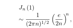
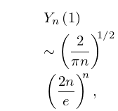
is satisfied by and , where and are the Bessel functions of the first kind. For large ,
| 3.6.12 | |||
| 3.6.13 | |||
(§10.19(i)). Thus is dominant and can be computed by forward recursion, whereas is recessive and has to be computed by backward recursion. The backward recursion can be carried out using independently computed values of and or by use of Miller’s algorithm (§3.6(iii)) or Olver’s algorithm (§3.6(v)).
Example 2. Weber Function
The Weber function satisfies
| 3.6.14 | |||
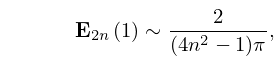
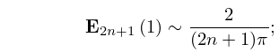
for , and as
| 3.6.15 | ||||
| 3.6.16 | ||||
see §11.11(ii). Thus the asymptotic behavior of the particular solution is intermediate to those of the complementary functions and ; moreover, the conditions for Olver’s algorithm are satisfied. We apply the algorithm to compute to 8S for the range , beginning with the value obtained from the Maclaurin series expansion (§11.10(iii)).
In the notation of §3.6(v) we have and . The least value of that satisfies (3.6.9) is found to be 16. The results of the computations are displayed in Table 3.6.1. The values of for are the wanted values of . (It should be observed that for , however, the are progressively poorer approximations to : the underlined digits are in error.)
| 0 | ||||||||
| 1 | ||||||||
| 2 | ||||||||
| 3 | ||||||||
| 4 | ||||||||
| 5 | ||||||||
| 6 | ||||||||
| 7 | ||||||||
| 8 | ||||||||
| 9 | ||||||||
| 10 | ||||||||
| 11 | ||||||||
| 12 | ||||||||
| 13 | ||||||||
| 14 | ||||||||
| 15 | ||||||||
| 16 | ||||||||
§3.6(vii) Linear Difference Equations of Other Orders
Similar considerations apply to the first-order equation
| 3.6.17 | |||
Thus in the inhomogeneous case it may sometimes be necessary to recur backwards to achieve stability. For analyses and examples see Gautschi (1997b).
For a difference equation of order (),
| 3.6.18 | |||
or for systems of first-order inhomogeneous equations, boundary-value methods are the rule rather than the exception. Typically conditions are prescribed at the beginning of the range, and conditions at the end. Here , and its actual value depends on the asymptotic behavior of the wanted solution in relation to those of the other solutions. Within this framework forward and backward recursion may be regarded as the special cases and , respectively.
