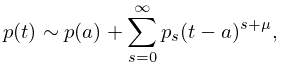
§2.3 Integrals of a Real Variable
Contents
- §2.3(i) Integration by Parts
- §2.3(ii) Watson’s Lemma
- §2.3(iii) Laplace’s Method
- §2.3(iv) Method of Stationary Phase
- §2.3(v) Coalescing Peak and Endpoint: Bleistein’s Method
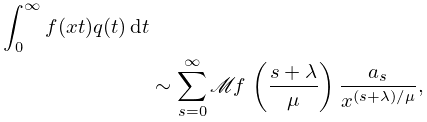
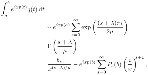
- §2.3(vi) Asymptotics of Mellin Transforms
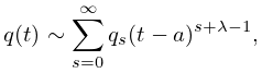
§2.3(i) Integration by Parts
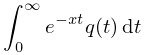
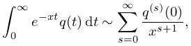
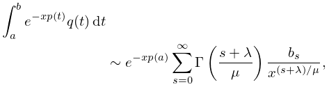
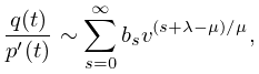
Assume that the Laplace transform
| 2.3.1 | |||
converges for all sufficiently large , and is infinitely differentiable in a neighborhood of the origin. Then
| 2.3.2 | |||
| . | |||
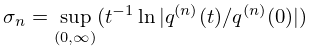
If, in addition, is infinitely differentiable on and
| 2.3.3 | |||
is finite and bounded for , then the th error term (that is, the difference between the integral and th partial sum in (2.3.2)) is bounded in absolute value by when exceeds both and .
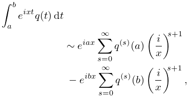
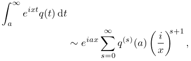
For the Fourier integral
assume and are finite, and is infinitely differentiable on . Then
| 2.3.4 | |||
| . | |||
Alternatively, assume , is infinitely differentiable on , and each of the integrals , , converges as uniformly for all sufficiently large . Then
| 2.3.5 | |||
| . | |||
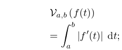
In both cases the th error term is bounded in absolute value by , where the variational operator is defined by
| 2.3.6 | |||
see §1.4(v). For other examples, see Wong (1989, Chapter 1).
§2.3(ii) Watson’s Lemma
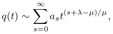
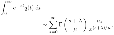
Assume again that the integral (2.3.1) converges for all sufficiently large , but now
| 2.3.7 | |||
| , | |||
where and are positive constants. Then the series obtained by substituting (2.3.7) into (2.3.1) and integrating formally term by term yields an asymptotic expansion:
| 2.3.8 | |||
| . | |||
For the function see §5.2(i).
This result is probably the most frequently used method for deriving asymptotic expansions of special functions. Since need not be continuous (as long as the integral converges), the case of a finite integration range is included. For an extension with more general -powers see Bleistein and Handelsman (1975, §4.1).
Other types of singular behavior in the integrand can be treated in an analogous manner. For example,
| 2.3.9 | |||
provided that the integral on the left-hand side of (2.3.9) converges for all sufficiently large values of . (In other words, differentiation of (2.3.8) with respect to the parameter (or ) is legitimate.)
§2.3(iii) Laplace’s Method
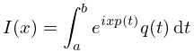
When is real and is a large positive parameter, the main contribution to the integral
| 2.3.13 | |||
derives from the neighborhood of the minimum of in the integration range. Without loss of generality, we assume that this minimum is at the left endpoint . Furthermore:
-
(a)
and are continuous in a neighborhood of , save possibly at , and the minimum of in is approached only at .
-
(b)
As
2.3.14 and the expansion for is differentiable. Again and are positive constants. Also (consistent with (a)).
-
(c)
The integral (2.3.13) converges absolutely for all sufficiently large .
Then
| 2.3.15 | |||
| , | |||
where the coefficients are defined by the expansion
| 2.3.16 | |||
| , | |||
in which . For example,
| 2.3.17 | ||||
In general
| 2.3.18 | |||
| . | |||
Watson’s lemma can be regarded as a special case of this result.
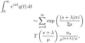
§2.3(iv) Method of Stationary Phase
When the parameter is large the contributions from the real and imaginary parts of the integrand in
| 2.3.19 | |||
oscillate rapidly and cancel themselves over most of the range. However, cancellation does not take place near the endpoints, owing to lack of symmetry, nor in the neighborhoods of zeros of because changes relatively slowly at these stationary points.
The first result is the analog of Watson’s lemma (§2.3(ii)). Assume that again has the expansion (2.3.7) and this expansion is infinitely differentiable, is infinitely differentiable on , and each of the integrals , , converges at , uniformly for all sufficiently large . Then
| 2.3.20 | |||
| , | |||
where the coefficients are given by (2.3.7).
For the more general integral (2.3.19) we assume, without loss of generality, that the stationary point (if any) is at the left endpoint. Furthermore:
-
(a)
On , and are infinitely differentiable and .
-
(b)
As the asymptotic expansions (2.3.14) apply, and each is infinitely differentiable. Again , , and are positive.
-
(c)
If the limit of as is finite, then each of the functions
2.3.21 , tends to a finite limit .
-
(d)
If , then and each of the integrals
2.3.22 , converges at uniformly for all sufficiently large .
If is finite, then both endpoints contribute:
| 2.3.23 | |||
| . | |||
But if (d) applies, then the second sum is absent. The coefficients are defined as in §2.3(iii).
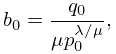
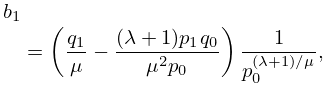
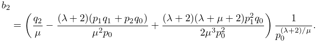
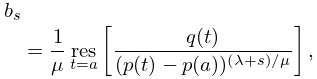
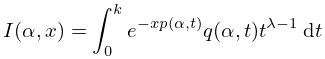
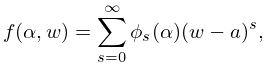
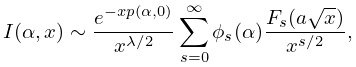
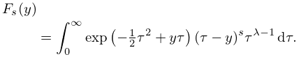
§2.3(v) Coalescing Peak and Endpoint: Bleistein’s Method
In the integral
| 2.3.24 | |||
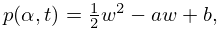
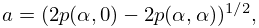
() and are positive constants, is a variable parameter in an interval with and , and is a large positive parameter. Assume also that and are continuous in and , and for each the minimum value of in is at , at which point vanishes, but both and are nonzero. When Laplace’s method (§2.3(iii)) applies, but the form of the resulting approximation is discontinuous at . In consequence, the approximation is nonuniform with respect to and deteriorates severely as .
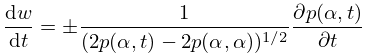
A uniform approximation can be constructed by quadratic change of integration variable:
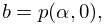
| 2.3.25 | |||
where and are functions of chosen in such a way that corresponds to , and the stationary points and correspond. Thus
| 2.3.26 | ||||
| 2.3.27 | |||
the upper or lower sign being taken according as . The relationship between and is one-to-one, and because
| 2.3.28 | |||
it is free from singularity at .
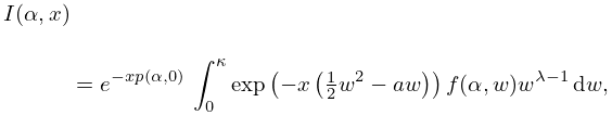
The integral (2.3.24) transforms into
| 2.3.29 | |||
where
| 2.3.30 | |||
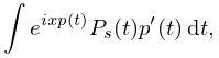
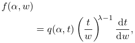
being the value of at . We now expand in a Taylor series centered at the peak value of the exponential factor in the integrand:
| 2.3.31 | |||
with the coefficients continuous at . The desired uniform expansion is then obtained formally as in Watson’s lemma and Laplace’s method. We replace the limit by and integrate term-by-term:
| 2.3.32 | |||
| , | |||
where
| 2.3.33 | |||
