§1.5 Calculus of Two or More Variables
Contents
- §1.5(i) Partial Derivatives
- §1.5(ii) Coordinate Systems
- §1.5(iii) Taylor’s Theorem; Maxima and Minima
- §1.5(iv) Leibniz’s Theorem for Differentiation of Integrals
- §1.5(v) Multiple Integrals
- §1.5(vi) Jacobians and Change of Variables
§1.5(i) Partial Derivatives
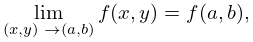
A function is continuous at a point if
| 1.5.1 | |||
that is, for every arbitrarily small positive constant there exists () such that
| 1.5.2 | |||
for all and that satisfy .
A function is continuous on a point set if it is continuous at all points of . A function is piecewise continuous on , where and are intervals, if it is piecewise continuous in for each and piecewise continuous in for each .
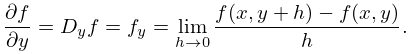
| 1.5.3 | ||||
| 1.5.4 | ||||
| 1.5.5 | ||||
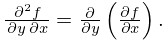
The function is continuously differentiable if , , and are continuous, and twice-continuously differentiable if also , , , and are continuous. In the latter event
| 1.5.6 | |||
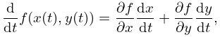
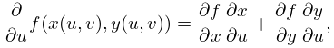
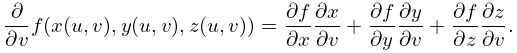
Chain Rule
| 1.5.7 | ||||
| 1.5.8 | ||||
| 1.5.9 | ||||
Implicit Function Theorem
If is continuously differentiable, , and at , then in a neighborhood of , that is, an open disk centered at , the equation defines a continuously differentiable function such that , , and .
§1.5(ii) Coordinate Systems
Notations
The notations given in this subsection, and also in other coordinate systems in the DLMF, are those generally used by physicists. For mathematicians the symbols and now are usually interchanged.
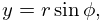
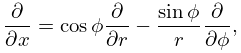
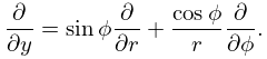
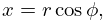
Polar Coordinates
With , ,
| 1.5.10 | ||||
| 1.5.11 | ||||
| 1.5.12 | ||||
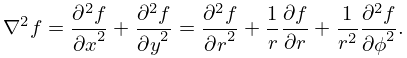
The Laplacian is given by
| 1.5.13 | |||
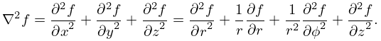
Cylindrical Coordinates
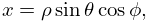
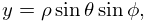
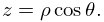
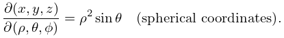
Spherical Coordinates
With , , ,
| 1.5.16 | ||||
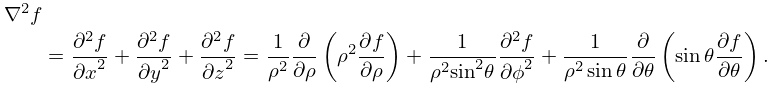
The Laplacian is given by
| 1.5.17 | |||
§1.5(iii) Taylor’s Theorem; Maxima and Minima
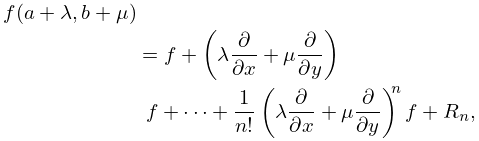
If is times continuously differentiable, then
| 1.5.18 | |||
where and its partial derivatives on the right-hand side are evaluated at , and as .
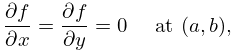
has a local minimum (maximum) at if
| 1.5.19 | |||
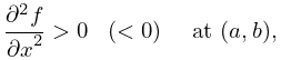
and the second order term in (1.5.18) is positive definite (negative definite), that is,
| 1.5.20 | |||
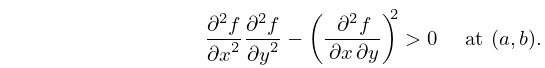
and
| 1.5.21 | |||
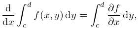
§1.5(iv) Leibniz’s Theorem for Differentiation of Integrals
Finite Integrals
| 1.5.22 | |||
Sufficient conditions for validity are: (a) and are continuous on a rectangle , ; (b) when both and are continuously differentiable and lie in .
Infinite Integrals
Suppose that are finite, is finite or , and , are continuous on the partly-closed rectangle or infinite strip . Suppose also that converges and converges uniformly on , that is, given any positive number , however small, we can find a number that is independent of and is such that
| 1.5.23 | |||
for all and all . Then
| 1.5.24 | |||
| . | |||
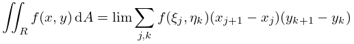
§1.5(v) Multiple Integrals
Double Integrals
Let be defined on a closed rectangle . For
| 1.5.25 | ||||
| 1.5.26 | ||||
let denote any point in the rectangle , , . Then the double integral of over is defined by
| 1.5.27 | |||
as . Sufficient conditions for the limit to exist are that is continuous, or piecewise continuous, on .
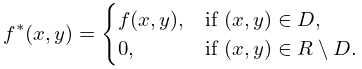
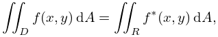
For defined on a point set contained in a rectangle , let
| 1.5.28 | |||
Then
| 1.5.29 | |||
provided the latter integral exists.
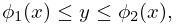
If is continuous, and is the set
| 1.5.30 | ||||
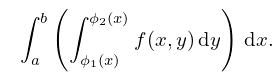
with and continuous, then
| 1.5.31 | |||
where the right-hand side is interpreted as the repeated integral
| 1.5.32 | |||
In particular, and can be constants.
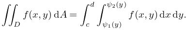
Similarly, if is the set
| 1.5.33 | ||||
with and continuous, then
| 1.5.34 | |||
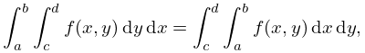
Change of Order of Integration
Infinite Double Integrals
Infinite double integrals occur when becomes infinite at points in or when is unbounded. In the cases (1.5.30) and (1.5.33) they are defined by taking limits in the repeated integrals (1.5.32) and (1.5.34) in an analogous manner to (1.4.22)–(1.4.23).
Moreover, if are finite or infinite constants and is piecewise continuous on the set , then
| 1.5.36 | |||
whenever both repeated integrals exist and at least one is absolutely convergent.
Triple Integrals
Finite and infinite integrals can be defined in a similar way. In case of triple integrals the sets are of the form
| 1.5.37 | ||||
A more general concept of integrability (both finite and infinite) for functions on domains in is Lebesgue integrability. See Rudin (1966).
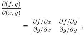
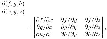
§1.5(vi) Jacobians and Change of Variables
Jacobian
| 1.5.38 | ||||
| 1.5.39 | ||||
| 1.5.40 | ||||
| 1.5.41 | ||||
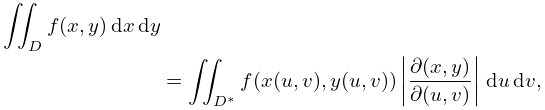
Change of Variables
| 1.5.42 | |||
where is the image of under a mapping which is one-to-one except perhaps for a set of points of area zero.
| 1.5.43 | |||
Again the mapping is one-to-one except perhaps for a set of points of volume zero.
