two or more variables

SearchAdvancedHelp

(0.003 seconds)

1—10 of 307 matching pages

1: 18.37 Classical OP’s in Two or More Variables

§18.37 Classical OP’s in Two or More Variables

…

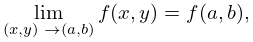
2: 1.5 Calculus of Two or More Variables

§1.5 Calculus of Two or More Variables

►

§1.5(i) Partial Derivatives

… ►

1.5.1 $$\underset{(x,y)\to (a,b)}{lim}f(x,y)=f(a,b),$$

ⓘ

Symbols:

$(a,b)$: open interval

Referenced by:

§1.9(ii)

Permalink:

http://dlmf.nist.gov/1.5.E1

Encodings:

pMML, png, TeX

See also:

Annotations for §1.5(i), §1.5 and Ch.1

… ►

§1.5(iii) Taylor’s Theorem; Maxima and Minima

… ►

3: 35.2 Laplace Transform

… ►where the integration variable $𝐗$ ranges over the space $𝛀$. …

4: 21.8 Abelian Functions

… ►In consequence, Abelian functions are generalizations of elliptic functions (§23.2(iii)) to more than one complex variable. …

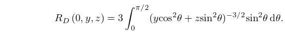
5: 19.23 Integral Representations

… ►

19.23.3 $$R_D(0,y,z)=3{\int }_0^{\pi /2}{(y{\cos }^2\theta +z{\sin }^2\theta )}^{-3/2}{\sin }^2\theta d\theta .$$

ⓘ

Symbols:

$R_D(x,y,z)$: elliptic integral symmetric in only two variables, $\pi$: the ratio of the circumference of a circle to its diameter, $\cos z$: cosine function, $dx$: differential of $x$ , $\int$: integral and $\sin z$: sine function

Referenced by:

§19.23, §19.23

Permalink:

http://dlmf.nist.gov/19.23.E3

Encodings:

pMML, png, TeX

See also:

Annotations for §19.23 and Ch.19

… ►In (19.23.8)–(19.23.10) one or more of the variables may be 0 if the integral converges. …

6: 37.3 Triangular Region with Weight Function

… ►

§37.3(i) Orthogonal Decomposition

… ►

37.3.1

ⓘ

Defines:

: weight function in two-variables on $\mathrm{△}$ (locally)

Symbols:

$\mathrm{△}$: triangular region, $x$: real variable, $y$: real variable, : real parameter ($>-1$), : real parameter ($>-1$) and : real parameter ($>-1$)

Referenced by:

§37.5(iii)

Permalink:

http://dlmf.nist.gov/37.3.E1

Encodings:

pMML, png, TeX

See also:

Annotations for §37.3(i), §37.3, Part 37.II and Ch.37

… ► … ►two further orthogonal bases of ${𝒱}_n^{\alpha ,\beta ,\gamma }$: … ►The biorthogonality of the two bases is given by …

7: Errata

… ►

The wording was changed to make the integration variable more apparent.

… ►

The symbol $\sim$ is used for two purposes in the DLMF, in some cases for asymptotic equality and in other cases for asymptotic expansion, but links to the appropriate definitions were not provided. In this release changes have been made to provide these links.

►

A short paragraph dealing with asymptotic approximations that are expressed in terms of two or more Poincaré asymptotic expansions has been added below (2.1.16).

… ►

Originally used $f(x)$ to represent both $U(-c,x)$ and $\overline{U}(-c,x)$. This has been replaced by two equations giving explicit definitions for the two envelope functions. Some slight changes in wording were needed to make this clear to readers.

… ►

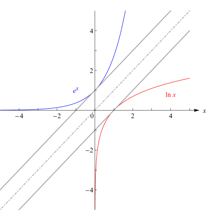
This figure was rescaled, with symmetry lines added, to make evident the symmetry due to the inverse relationship between the two functions.

Reported 2015-11-12 by James W. Pitman.

…

8: 33.22 Particle Scattering and Atomic and Molecular Spectra

… ►With $\mathrm{e}$ denoting here the elementary charge, the Coulomb potential between two point particles with charges $Z_1\mathrm{e},Z_2\mathrm{e}$ and masses $m_1,m_2$ separated by a distance $s$ is $V(s)=Z_1{Z}_2{\mathrm{e}}^2/(4\pi {\epsilon }_{0}s)=Z_1{Z}_2\alpha \mathrm{\hslash }c/s$, where $Z_j$ are atomic numbers, ${\epsilon }_0$ is the electric constant, $\alpha$ is the fine structure constant, and $\mathrm{\hslash }$ is the reduced Planck’s constant. … ►In these applications, the $Z$-scaled variables $r$ and $ϵ$ are more convenient. …

9: 37.2 General Orthogonal Polynomials of Two Variables

§37.2 General Orthogonal Polynomials of Two Variables

… ► … ► … ►

§37.2(iii) Reproducing Kernels

… ►

§37.2(iv) Zeros

…

10: Sidebar 21.SB2: A two-phase solution of the Kadomtsev–Petviashvili equation (21.9.3)

Sidebar 21.SB2: A two-phase solution of the Kadomtsev–Petviashvili equation (21.9.3)

… ►A two-phase solution of the Kadomtsev–Petviashvili equation (21.9.3). Such a solution is given in terms of a Riemann theta function with two phases. …The agreement of these solutions with two-dimensional surface water waves in shallow water was considered in Hammack et al. (1989, 1995).