local

SearchAdvancedHelp

(0.001 seconds)

1—10 of 199 matching pages

1: 31.3 Basic Solutions

… ► $H\mathrm{\ell }(a,q;\alpha ,\beta ,\gamma ,\delta ;z)$ denotes the solution of (31.2.1) that corresponds to the exponent $0$ at $z=0$ and assumes the value $1$ there. If the other exponent is not a positive integer, that is, if $\gamma \ne 0,-1,-2,\mathrm{\dots }$, then from §2.7(i) it follows that $H\mathrm{\ell }(a,q;\alpha ,\beta ,\gamma ,\delta ;z)$ exists, is analytic in the disk , and has the Maclaurin expansion … ►Solutions (31.3.1) and (31.3.5)–(31.3.11) comprise a set of 8 local solutions of (31.2.1): 2 per singular point. …For example, $H\mathrm{\ell }(a,q;\alpha ,\beta ,\gamma ,\delta ;z)$ is equal to … ►The full set of 192 local solutions of (31.2.1), equivalent in 8 sets of 24, resembles Kummer’s set of 24 local solutions of the hypergeometric equation, which are equivalent in 4 sets of 6 solutions (§15.10(ii)); see Maier (2007).

2: 4.42 Solution of Triangles

…

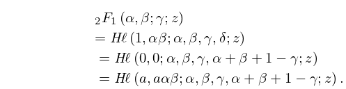
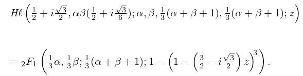
3: 31.7 Relations to Other Functions

… ►

31.7.1 $${}_2{}^{}F_1^{}(\alpha ,\beta ;\gamma ;z)=H\mathrm{\ell }(1,\alpha \beta ;\alpha ,\beta ,\gamma ,\delta ;z)=H\mathrm{\ell }(0,0;\alpha ,\beta ,\gamma ,\alpha +\beta +1-\gamma ;z)=H\mathrm{\ell }(a,a\alpha \beta ;\alpha ,\beta ,\gamma ,\alpha +\beta +1-\gamma ;z).$$

ⓘ

Symbols:

${}_2{}^{}F_1^{}(a,b;c;z)$: $=F(a,b;c;z)$ notation for Gauss’ hypergeometric function, $H\mathrm{\ell }(a,q;\alpha ,\beta ,\gamma ,\delta ;z)$: Heun functions, $z$: complex variable, $\gamma$: real or complex parameter, $\delta$: real or complex parameter, $a$: complex parameter, $\alpha$: real or complex parameter and $\beta$: real or complex parameter

Permalink:

http://dlmf.nist.gov/31.7.E1

Encodings:

pMML, png, TeX

See also:

Annotations for §31.7(i), §31.7 and Ch.31

►Other reductions of $H\mathrm{\ell }$ to a ${}_2{}^{}F_1^{}$, with at least one free parameter, exist iff the pair $(a,p)$ takes one of a finite number of values, where $q=\alpha \beta p$. … ►

31.7.2 $$H\mathrm{\ell }(2,\alpha \beta ;\alpha ,\beta ,\gamma ,\alpha +\beta -2\gamma +1;z)={}_2{}^{}F_1^{}(\frac{1}{2}\alpha ,\frac{1}{2}\beta ;\gamma ;1-{(1-z)}^2),$$

ⓘ

Symbols:

${}_2{}^{}F_1^{}(a,b;c;z)$: $=F(a,b;c;z)$ notation for Gauss’ hypergeometric function, $H\mathrm{\ell }(a,q;\alpha ,\beta ,\gamma ,\delta ;z)$: Heun functions, $z$: complex variable, $\gamma$: real or complex parameter, $\alpha$: real or complex parameter and $\beta$: real or complex parameter

Permalink:

http://dlmf.nist.gov/31.7.E2

Encodings:

pMML, png, TeX

See also:

Annotations for §31.7(i), §31.7 and Ch.31

►

31.7.3 $$H\mathrm{\ell }(4,\alpha \beta ;\alpha ,\beta ,\frac{1}{2},\frac{2}{3}(\alpha +\beta );z)={}_2{}^{}F_1^{}(\frac{1}{3}\alpha ,\frac{1}{3}\beta ;\frac{1}{2};1-{(1-z)}^2(1-\frac{1}{4}z)),$$

ⓘ

Symbols:

${}_2{}^{}F_1^{}(a,b;c;z)$: $=F(a,b;c;z)$ notation for Gauss’ hypergeometric function, $H\mathrm{\ell }(a,q;\alpha ,\beta ,\gamma ,\delta ;z)$: Heun functions, $z$: complex variable, $\alpha$: real or complex parameter and $\beta$: real or complex parameter

Permalink:

http://dlmf.nist.gov/31.7.E3

Encodings:

pMML, png, TeX

See also:

Annotations for §31.7(i), §31.7 and Ch.31

►

31.7.4 $$H\mathrm{\ell }(\frac{1}{2}+\mathrm{i}\frac{\sqrt{3}}{2},\alpha \beta (\frac{1}{2}+\mathrm{i}\frac{\sqrt{3}}{6});\alpha ,\beta ,\frac{1}{3}(\alpha +\beta +1),\frac{1}{3}(\alpha +\beta +1);z)={}_2{}^{}F_1^{}(\frac{1}{3}\alpha ,\frac{1}{3}\beta ;\frac{1}{3}(\alpha +\beta +1);1-{\left(1-\left(\frac{3}{2}-\mathrm{i}\frac{\sqrt{3}}{2}\right)z\right)}^3).$$

ⓘ

Symbols:

${}_2{}^{}F_1^{}(a,b;c;z)$: $=F(a,b;c;z)$ notation for Gauss’ hypergeometric function, $H\mathrm{\ell }(a,q;\alpha ,\beta ,\gamma ,\delta ;z)$: Heun functions, $\mathrm{i}$: imaginary unit, $z$: complex variable, $\alpha$: real or complex parameter and $\beta$: real or complex parameter

Permalink:

http://dlmf.nist.gov/31.7.E4

Encodings:

pMML, png, TeX

See also:

Annotations for §31.7(i), §31.7 and Ch.31

…

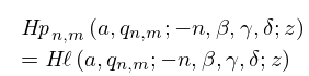
4: 31.5 Solutions Analytic at Three Singularities: Heun Polynomials

… ►

31.5.2 $${\mathrm{𝐻𝑝}}_{n,m}(a,q_{n,m};-n,\beta ,\gamma ,\delta ;z)=H\mathrm{\ell }(a,q_{n,m};-n,\beta ,\gamma ,\delta ;z)$$

ⓘ

Defines:

${\mathrm{𝐻𝑝}}_{n,m}(a,q_{n,m};-n,\beta ,\gamma ,\delta ;z)$: Heun polynomials

Symbols:

$H\mathrm{\ell }(a,q;\alpha ,\beta ,\gamma ,\delta ;z)$: Heun functions, $z$: complex variable, $\gamma$: real or complex parameter, $\delta$: real or complex parameter, $m$: nonnegative integer, $n$: nonnegative integer, $a$: complex parameter, $q$: real or complex parameter and $\beta$: real or complex parameter

Permalink:

http://dlmf.nist.gov/31.5.E2

Encodings:

pMML, png, TeX

See also:

Annotations for §31.5 and Ch.31

…

5: 31.1 Special Notation

… ►The main functions treated in this chapter are $H\mathrm{\ell }(a,q;\alpha ,\beta ,\gamma ,\delta ;z)$, $(s_1,s_2){\mathrm{𝐻𝑓}}_m(a,q_m;\alpha ,\beta ,\gamma ,\delta ;z)$, $(s_1,s_2){\mathrm{𝐻𝑓}}_m^{\nu }(a,q_m;\alpha ,\beta ,\gamma ,\delta ;z)$, and the polynomial ${\mathrm{𝐻𝑝}}_{n,m}(a,q_{n,m};-n,\beta ,\gamma ,\delta ;z)$. …

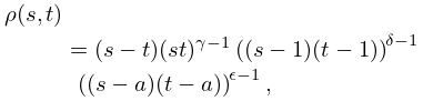
6: 31.9 Orthogonality

… ►

31.9.3 $${\theta }_m={(1-{\mathrm{e}}^{2\pi \mathrm{i}\gamma })(1-{\mathrm{e}}^{2\pi \mathrm{i}\delta }){\zeta }^{\gamma }{(1-\zeta )}^{\delta }{(\zeta -a)}^{ϵ}\frac{f_0(q,\zeta )}{f_1(q,\zeta )}\frac{\partial }{\partial q}𝒲\left\{f_0(q,\zeta ),f_1(q,\zeta )\right\}|}_{q=q_m},$$

ⓘ

Defines:

${\theta }_m$: normalization constant (locally)

Symbols:

$𝒲$: Wronskian, $\pi$: the ratio of the circumference of a circle to its diameter, $\mathrm{e}$: base of natural logarithm, $\mathrm{i}$: imaginary unit, $\frac{\partial f}{\partial x}$: partial derivative of $f$ with respect to $x$ , $\partial x$: partial differential of $x$ , $\gamma$: real or complex parameter, $\delta$: real or complex parameter, $ϵ$: real or complex parameter, $m$: nonnegative integer, $a$: complex parameter, $q$: real or complex parameter, $\zeta$: point and $f_0(q_m,z)$, $f_1(q_m,z)$: coefficients

Permalink:

http://dlmf.nist.gov/31.9.E3

Encodings:

pMML, png, TeX

See also:

Annotations for §31.9(i), §31.9 and Ch.31

… ►

$$f_0(q_m,z)=H\mathrm{\ell }(a,q_m;\alpha ,\beta ,\gamma ,\delta ;z),$$

►

$$f_1(q_m,z)=H\mathrm{\ell }(1-a,\alpha \beta -q_m;\alpha ,\beta ,\delta ,\gamma ;1-z),$$

… ►

31.9.6 $$\rho (s,t)=(s-t){(st)}^{\gamma -1}{\left((s-1)(t-1)\right)}^{\delta -1}{\left((s-a)(t-a)\right)}^{ϵ-1},$$

ⓘ

Defines:

$\rho (s,t)$: weight function (locally)

Symbols:

$\gamma$: real or complex parameter, $\delta$: real or complex parameter, $ϵ$: real or complex parameter and $a$: complex parameter

Permalink:

http://dlmf.nist.gov/31.9.E6

Encodings:

pMML, png, TeX

See also:

Annotations for §31.9(ii), §31.9 and Ch.31

…

7: 2.6 Distributional Methods

… ►Let $f(t)$ be locally integrable on $[0,\mathrm{\infty })$. The Stieltjes transform of $f(t)$ is defined by …Since $f(t)$ is locally integrable on $[0,\mathrm{\infty })$, it defines a distribution by … ►In terms of the convolution product …of two locally integrable functions on $[0,\mathrm{\infty })$, (2.6.33) can be written …

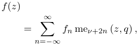
8: 28.19 Expansions in Series of ${\mathrm{me}}_{\nu +2n}$ Functions

… ►

28.19.2 $$f(z)=\sum _{n=-\mathrm{\infty }}^{\mathrm{\infty }}{f}_n{\mathrm{me}}_{\nu +2n}(z,q),$$

ⓘ

Defines:

$f(z)$: function (locally)

Symbols:

${\mathrm{me}}_n(z,q)$: Mathieu function, $q=h^2$: parameter, $n$: integer, $z$: complex variable, $\nu$: complex parameter and $f_n$: coefficients

Referenced by:

§28.19

Permalink:

http://dlmf.nist.gov/28.19.E2

Encodings:

pMML, png, TeX

See also:

Annotations for §28.19 and Ch.28

… ►

28.19.3 $$f_n=\frac{1}{\pi }{\int }_0^{\pi }f(z){\mathrm{me}}_{\nu +2n}(-z,q)dz.$$

ⓘ

Defines:

$f_n$: coefficients (locally)

Symbols:

${\mathrm{me}}_n(z,q)$: Mathieu function, $\pi$: the ratio of the circumference of a circle to its diameter, $dx$: differential of $x$ , $\int$: integral, $q=h^2$: parameter, $n$: integer, $z$: complex variable, $\nu$: complex parameter and $f(z)$: function

Permalink:

http://dlmf.nist.gov/28.19.E3

Encodings:

pMML, png, TeX

See also:

Annotations for §28.19 and Ch.28

…

9: 33.11 Asymptotic Expansions for Large $\rho$

…

10: 10.58 Zeros

…