double
(0.001 seconds)
1—10 of 93 matching pages
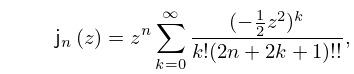
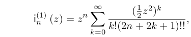
1: 10.53 Power Series
2: Bibliography Q
…
►
A new lower bound in the second Kershaw’s double inequality.
J. Comput. Appl. Math. 214 (2), pp. 610–616.
…
►
Uniform asymptotic expansions of a double integral: Coalescence of two stationary points.
Proc. Roy. Soc. London Ser. A 456, pp. 407–431.
…
3: Gerhard Wolf
…
► Schmidt) of the Chapter Double Confluent Heun
Equation in the book Heun’s Differential Equations (A.
…
4: 10.72 Mathematical Applications
…
►If has a double zero , or more generally is a zero of order , , then uniform asymptotic approximations (but not expansions) can be constructed in terms of Bessel functions, or modified Bessel functions, of order .
The number can also be replaced by any real constant
in the sense that
is analytic and nonvanishing at ; moreover, is permitted to have a single or double pole at .
The order of the approximating Bessel functions, or modified Bessel functions, is , except in the case when has a double pole at .
…
►
§10.72(iii) Differential Equations with a Double Pole and a Movable Turning Point
►In (10.72.1) assume and depend continuously on a real parameter , has a simple zero and a double pole , except for a critical value , where . …5: 27.5 Inversion Formulas
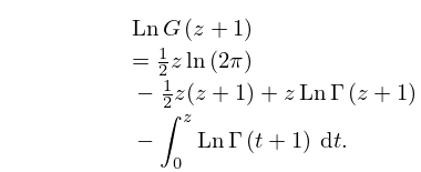
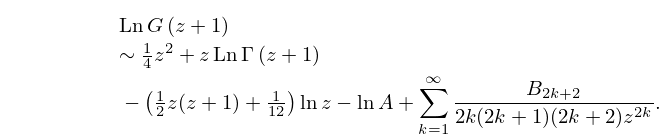
6: 5.17 Barnes’ -Function (Double Gamma Function)
7: 35.10 Methods of Computation
…
►Other methods include numerical quadrature applied to double and multiple integral representations.
…
8: 10.41 Asymptotic Expansions for Large Order
…
►
§10.41(iv) Double Asymptotic Properties
… ►§10.41(v) Double Asymptotic Properties (Continued)
…9: 10.52 Limiting Forms
10: 5.1 Special Notation
…
►
