three j symbols
(0.003 seconds)
11—18 of 18 matching pages
11: Errata
…
►
Chapters 10 Bessel Functions, 18 Orthogonal Polynomials, 34 3j, 6j, 9j Symbols
…
►
Subsection 5.2(iii)
…
►
Section 34.1
…
►
Section 34.1
…
►
Equation (34.7.4)
…
Three new identities for Pochhammer’s symbol (5.2.6)–(5.2.8) have been added at the end of this subsection.
Suggested by Tom Koornwinder.
The relation between Clebsch-Gordan and symbols was clarified, and the sign of was changed for readability. The reference Condon and Shortley (1935) for the Clebsch-Gordan coefficients was replaced by Edmonds (1974) and Rotenberg et al. (1959) and the references for , , symbols were made more precise in §34.1.
34.7.4
Originally the third symbol in the summation was written incorrectly as
Reported 2015-01-19 by Yan-Rui Liu.
12: 18.35 Pollaczek Polynomials
…
►The three types of Pollaczek polynomials were successively introduced in Pollaczek (1949a, b, 1950), see also Erdélyi et al. (1953b, p.219) and, for type 1 and 2, Szegö (1950) and Askey (1982b).
…
►
18.35.2_2
…
►
18.35.4_5
…
►More generally, the are OP’s if and only if one of the following three conditions holds (in case (iii) work with the monic polynomials (18.35.2_2)).
…
►
18.35.6_5
…
13: 18.27 -Hahn Class
…
►The generic (top level) cases are the -Hahn polynomials and the big -Jacobi polynomials, each of which depends on three further parameters.
…
►
18.27.4
,
…
►
18.27.14
,
…
►
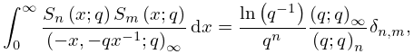
18.27.19
…
►
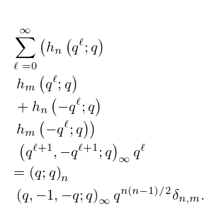
18.27.22
…
14: Bibliography T
…
►
Improved error bounds for the Liouville-Green (or WKB) approximation.
J. Math. Anal. Appl. 85 (1), pp. 79–89.
►
The Askey scheme for hypergeometric orthogonal polynomials viewed from asymptotic analysis.
J. Comput. Appl. Math. 133 (1-2), pp. 623–633.
…
►
Asymptotic expansions of Kummer hypergeometric functions with three asymptotic parameters a, b and z.
Indagationes Mathematicae.
…
►
Angular Momentum: An Illustrated Guide to Rotational Symmetries for Physical Systems.
A Wiley-Interscience Publication, John Wiley & Sons Inc., New York.
…
►
Evaluation of the exponential integral for large complex arguments.
J. Research Nat. Bur. Standards 52, pp. 313–317.
…
15: 19.29 Reduction of General Elliptic Integrals
…
►There are only three distinct ’s with subscripts , and at most one of them can be 0 because the ’s are nonzero.
…
►The advantages of symmetric integrals for tables of integrals and symbolic integration are illustrated by (19.29.4) and its cubic case, which replace the formulas in Gradshteyn and Ryzhik (2000, 3.147, 3.131, 3.152) after taking as the variable of integration in 3.
…
►where is an -tuple with 1 in the th position and 0’s elsewhere.
…
►Next, for , define , and assume both ’s are positive for .
…where
…
16: Mathematical Introduction
…
►The first three chapters of the NIST Handbook and DLMF are methodology chapters that provide detailed coverage of, and references for, mathematical topics that are especially important in the theory, computation, and application of special functions.
…
►
►
►
►
…
► J.
…
| complex plane (excluding infinity). | |
| … | |
| or | Kronecker delta: 0 if ; 1 if . |
| … | |
| or | half-closed intervals. |
|---|---|
| … | |
| or | matrix with th element or . |
| … | |
| Pochhammer’s symbol: if ; 1 if . | |
| … | |
17: Bibliography D
…
►
Computational properties of three-term recurrence relations for Kummer functions.
J. Comput. Appl. Math. 233 (6), pp. 1505–1510.
…
►
Texas Instruments, Inc..
…
►
Integral representations for elliptic functions.
J. Math. Anal. Appl. 316 (1), pp. 142–160.
…
►
Oscillatory integrals, Lagrange immersions and unfolding of singularities.
Comm. Pure Appl. Math. 27, pp. 207–281.
…
►
Novel identities for simple -
symbols.
J. Mathematical Phys. 16, pp. 318–319.
…
18: 18.39 Applications in the Physical Sciences
…
►Here are three examples of solutions for (18.39.8) for explicit choices of and with the corresponding to the discrete spectrum.
All are written in the same form as the product of three factors: the square root of a weight function , the corresponding OP or EOP, and constant factors ensuring unit normalization.
…
►
