§18.27(i) Introduction
The -hypergeometric OP’s comprise the -Hahn class
(or -linear lattice class) OP’s and the
Askey–Wilson class (or -quadratic lattice class) OP’s (§18.28).
Together they form the -Askey scheme.
This scheme gives a graphical
representation of all families of OP’s belonging to it together with the
limit relations between them, see
Koekoek et al. (2010, p. 414).
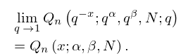
For the notation of -hypergeometric functions see §§17.2 and 17.4(i).
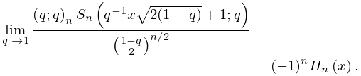
Unless said otherwise, we will assume that .
For (17.4.1) with , , and
we will use the convention
that the summation on the right-hand side ends at .
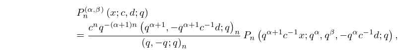
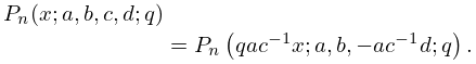
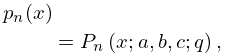
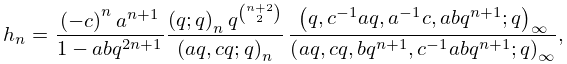
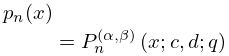
The -Hahn class OP’s comprise systems of OP’s ,
, or , that are eigenfunctions of a
second order -difference operator. Thus
| 18.27.1 |
|
|
|
|
|
where , , and are independent of , and where the
are the eigenvalues. In the -Hahn class OP’s the role of the
operator in the Jacobi, Laguerre, and Hermite cases is played
by the -derivative , as defined in (17.2.41). A
(nonexhaustive) classification of such systems of OP’s was made by
Hahn (1949). There are 18 families of OP’s of -Hahn class. These
families depend on further parameters, in addition to . The generic (top
level) cases are the -Hahn polynomials and the big -Jacobi polynomials,
each of which depends on three further parameters.
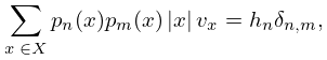
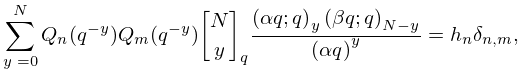
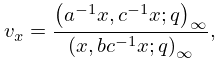
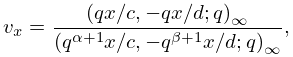
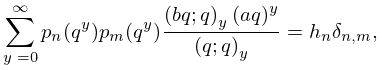
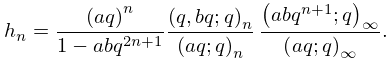
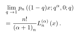
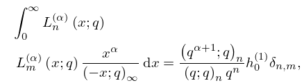
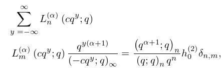
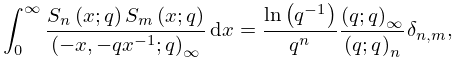
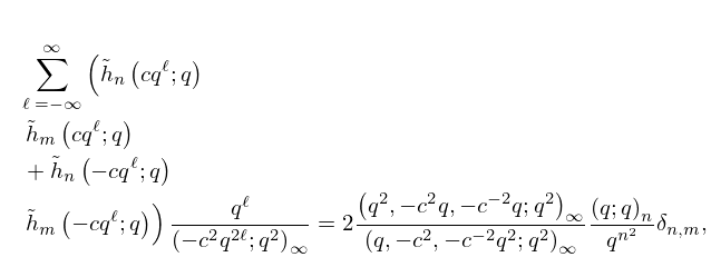
All these systems of OP’s have orthogonality properties of the form
| 18.27.2 |
|
|
|
|
|
where is given by or
. Here are fixed
positive real numbers, and and are sequences of successive integers,
finite or unbounded in one direction, or unbounded in both directions. If
and are both nonempty, then they are both unbounded to the right.
In case of unbounded sequences (18.27.2) can be rewritten as a
-integral, see §17.2(v),
and more generally Gasper and Rahman (2004, (1.11.2)).
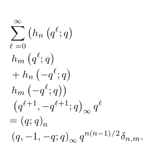
Some of the systems of OP’s that occur in the classification do not have a unique
orthogonality property. Thus in addition to a relation of the form
(18.27.2), such systems may also satisfy orthogonality relations
with respect to a continuous weight function on some interval.
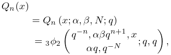
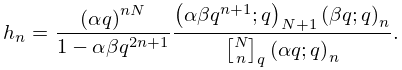
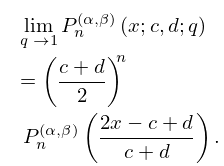
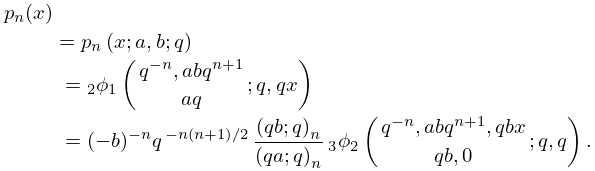
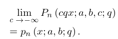
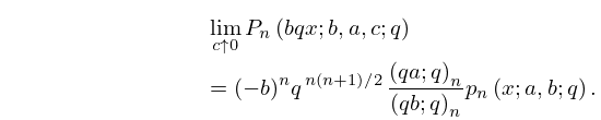
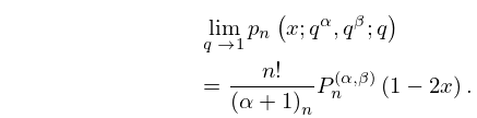
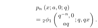
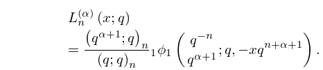
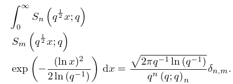
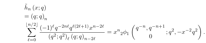
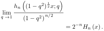
Here only a few families are mentioned. They are defined by their
-hypergeometric representations, followed by their orthogonality properties.
For other formulas, including -difference equations, recurrence relations,
duality formulas, special cases, and limit relations, see
Koekoek et al. (2010, Chapter 14). See also
Gasper and Rahman (2004, pp. 195–199, 228–230) and
Ismail (2009, Chapters 13, 18, 21).
