Laguerre

SearchAdvancedHelp

(0.001 seconds)

11—20 of 53 matching pages

11: 18.1 Notation

… ►

Classical OP’s

… ►

Laguerre: $L_n^{(\alpha )}\left(x\right)$ and $L_n\left(x\right)=L_n^{(0)}\left(x\right)$. ($L_n^{(\alpha )}\left(x\right)$ with $\alpha \ne 0$ is also called Generalized Laguerre.)

… ►

$q$-Laguerre: $L_n^{(\alpha )}(x;q)$.

…

12: 18.9 Recurrence Relations and Derivatives

… ►

Laguerre

►

18.9.13 $$L_n^{(\alpha )}\left(x\right)=L_n^{(\alpha +1)}\left(x\right)-L_{n-1}^{(\alpha +1)}\left(x\right),$$

ⓘ

Symbols:

$L_n^{(\alpha )}\left(x\right)$: Laguerre (or generalized Laguerre) polynomial, $n$: nonnegative integer and $x$: real variable

A&S Ref:

22.7.30

Referenced by:

§18.17(i), §18.9(ii), §18.9(ii)

Permalink:

http://dlmf.nist.gov/18.9.E13

Encodings:

pMML, png, TeX

See also:

Annotations for §18.9(ii), §18.9(ii), §18.9 and Ch.18

►

18.9.14 $$x{L}_n^{(\alpha +1)}\left(x\right)=-(n+1)L_{n+1}^{(\alpha )}\left(x\right)+(n+\alpha +1)L_n^{(\alpha )}\left(x\right).$$

ⓘ

Symbols:

$L_n^{(\alpha )}\left(x\right)$: Laguerre (or generalized Laguerre) polynomial, $n$: nonnegative integer and $x$: real variable

A&S Ref:

22.7.31

Referenced by:

§18.9(ii), §18.9(ii)

Permalink:

http://dlmf.nist.gov/18.9.E14

Encodings:

pMML, png, TeX

See also:

Annotations for §18.9(ii), §18.9(ii), §18.9 and Ch.18

… ►

Laguerre

… ►Further $n$-th derivative formulas relating two different Laguerre polynomials can be obtained from §13.3(ii) by substitution of (13.6.19). …

13: 8.7 Series Expansions

§8.7 Series Expansions

►For the functions $e_n(z)$, ${𝗂}_n^{(1)}\left(z\right)$, and $L_n^{(\alpha )}\left(x\right)$ see (8.4.11), §§10.47(ii), and 18.3, respectively. … ►

8.7.6 $$\mathrm{\Gamma }(a,x)=x^a{\mathrm{e}}^{-x}\sum _{n=0}^{\mathrm{\infty }}\frac{L_n^{(a)}\left(x\right)}{n+1},$$ $x>0$, .

ⓘ

Symbols:

$L_n^{(\alpha )}\left(x\right)$: Laguerre (or generalized Laguerre) polynomial, $\mathrm{e}$: base of natural logarithm, $\mathrm{\Gamma }(a,z)$: incomplete gamma function, $\mathrm{\Re }$: real part, $x$: real variable, $z$: complex variable, $a$: parameter and $n$: nonnegative integer

Proof sketch:

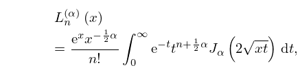
Integrate (18.12.13) from $z=0$ to $z=1$ and for the integral on the left-hand side use the substitution $z=\frac{t}{1+t}$. The resulting integral is (8.6.5). The constraint follows from (18.15.14).

Referenced by:

Erratum (V1.1.8) for Equation (8.7.6)

Permalink:

http://dlmf.nist.gov/8.7.E6

Encodings:

pMML, png, TeX

Addition (effective with 1.1.8):

The constraint was updated to include .

Suggested 2022-10-14 by Walter Gautschi

See also:

Annotations for §8.7 and Ch.8

…

14: 18.5 Explicit Representations

§18.5 Explicit Representations

… ►

Laguerre

… ►Similarly in the cases of the ultraspherical polynomials $C_n^{(\lambda )}\left(x\right)$ and the Laguerre polynomials $L_n^{(\alpha )}\left(x\right)$ we assume that $\lambda >-\frac{1}{2},\lambda \ne 0$, and $\alpha >-1$, unless stated otherwise. … ►

Laguerre

… ►

15: 18.21 Hahn Class: Interrelations

… ►

Meixner $\to$ Laguerre

►

18.21.8 $$\underset{c\to 1}{lim}{M}_n({(1-c)}^{-1}x;\alpha +1,c)=\frac{L_n^{(\alpha )}\left(x\right)}{L_n^{(\alpha )}\left(0\right)}.$$

ⓘ

Symbols:

$L_n^{(\alpha )}\left(x\right)$: Laguerre (or generalized Laguerre) polynomial, $M_n(x;\beta ,c)$: Meixner polynomial, $n$: nonnegative integer and $x$: real variable

Referenced by:

§18.21(ii)

Permalink:

http://dlmf.nist.gov/18.21.E8

Encodings:

pMML, png, TeX

See also:

Annotations for §18.21(ii), §18.21(ii), §18.21 and Ch.18

… ►

Meixner–Pollaczek $\to$ Laguerre

►

18.21.12 $$\underset{\varphi \to 0}{lim}{P}_n^{(\frac{1}{2}\alpha +\frac{1}{2})}(-{(2\varphi )}^{-1}x;\varphi )=L_n^{(\alpha )}\left(x\right).$$

ⓘ

Symbols:

$L_n^{(\alpha )}\left(x\right)$: Laguerre (or generalized Laguerre) polynomial, $P_n^{(\lambda )}(x;\varphi )$: Meixner–Pollaczek polynomial, $n$: nonnegative integer and $x$: real variable

Referenced by:

§18.21(ii), §18.24, §18.30(v)

Permalink:

http://dlmf.nist.gov/18.21.E12

Encodings:

pMML, png, TeX

See also:

Annotations for §18.21(ii), §18.21(ii), §18.21 and Ch.18

… ►

►►

Figure 18.21.1: Askey scheme. … Magnify

16: 18.10 Integral Representations

… ►

Laguerre

… ►for the Jacobi, Laguerre, and Hermite polynomials. … ►

Table 18.10.1: Classical OP’s: contour integral representations (18.10.8).

► ►►

$p_n(x)$	$g_0(x)$	$g_1(z,x)$	$g_2(z,x)$	$c$	Conditions
…

►

… ►

Laguerre

►

18.10.9 $$L_n^{(\alpha )}\left(x\right)=\frac{{\mathrm{e}}^x{x}^{-\frac{1}{2}\alpha }}{n!}{\int }_0^{\mathrm{\infty }}{\mathrm{e}}^{-t}{t}^{n+\frac{1}{2}\alpha }{J}_{\alpha }\left(2\sqrt{xt}\right)dt,$$ $\alpha >-1$.

ⓘ

Symbols:

$J_{\nu }\left(z\right)$: Bessel function of the first kind, $L_n^{(\alpha )}\left(x\right)$: Laguerre (or generalized Laguerre) polynomial, $dx$: differential of $x$ , $\mathrm{e}$: base of natural logarithm, $!$: factorial (as in $n!$), $\int$: integral, $t$: real variable, $n$: nonnegative integer and $x$: real variable

A&S Ref:

22.10.14

Referenced by:

§18.10(iv)

Permalink:

http://dlmf.nist.gov/18.10.E9

Encodings:

pMML, png, TeX

See also:

Annotations for §18.10(iv), §18.10(iv), §18.10 and Ch.18

…

17: 18.7 Interrelations and Limit Relations

… ►

18.7.19 $$H_{2n}\left(x\right)={(-1)}^n{2}^{2n}n!L_n^{(-\frac{1}{2})}\left(x^2\right),$$

ⓘ

Symbols:

$H_n\left(x\right)$: Hermite polynomial, $L_n^{(\alpha )}\left(x\right)$: Laguerre (or generalized Laguerre) polynomial, $!$: factorial (as in $n!$), $n$: nonnegative integer and $x$: real variable

A&S Ref:

22.5.40

Referenced by:

§18.16(v), §18.18(iii), §18.18(iv), §18.18(viii), §18.7(ii)

Permalink:

http://dlmf.nist.gov/18.7.E19

Encodings:

pMML, png, TeX

See also:

Annotations for §18.7(ii), §18.7 and Ch.18

►

18.7.20 $$H_{2n+1}\left(x\right)={(-1)}^n{2}^{2n+1}n!x{L}_n^{(\frac{1}{2})}\left(x^2\right).$$

ⓘ

Symbols:

$H_n\left(x\right)$: Hermite polynomial, $L_n^{(\alpha )}\left(x\right)$: Laguerre (or generalized Laguerre) polynomial, $!$: factorial (as in $n!$), $n$: nonnegative integer and $x$: real variable

A&S Ref:

22.5.41

Referenced by:

§18.16(v), §18.18(iii), §18.18(iv), §18.7(ii), §18.7(ii)

Permalink:

http://dlmf.nist.gov/18.7.E20

Encodings:

pMML, png, TeX

See also:

Annotations for §18.7(ii), §18.7 and Ch.18

… ►

Jacobi $\to$ Laguerre

►

18.7.21 $$\underset{\beta \to \mathrm{\infty }}{lim}{P}_n^{(\alpha ,\beta )}\left(1-\left(2x/\beta \right)\right)=L_n^{(\alpha )}\left(x\right).$$

ⓘ

Symbols:

$P_n^{(\alpha ,\beta )}\left(x\right)$: Jacobi polynomial, $L_n^{(\alpha )}\left(x\right)$: Laguerre (or generalized Laguerre) polynomial, $n$: nonnegative integer and $x$: real variable

A&S Ref:

22.15.5

Referenced by:

§18.10(ii), §18.7(iii)

Permalink:

http://dlmf.nist.gov/18.7.E21

Encodings:

pMML, png, TeX

See also:

Annotations for §18.7(iii), §18.7(iii), §18.7 and Ch.18

… ►

Laguerre $\to$ Hermite

…

18: 18.11 Relations to Other Functions

… ►

Laguerre

►

18.11.2 $$L_n^{(\alpha )}\left(x\right)=\frac{{\left(\alpha +1\right)}_n}{n!}M(-n,\alpha +1,x)=\frac{{(-1)}^n}{n!}U(-n,\alpha +1,x)=\frac{{\left(\alpha +1\right)}_n}{n!}{x}^{-\frac{1}{2}(\alpha +1)}{\mathrm{e}}^{\frac{1}{2}x}{M}_{n+\frac{1}{2}(\alpha +1),\frac{1}{2}\alpha }\left(x\right)=\frac{{(-1)}^n}{n!}{x}^{-\frac{1}{2}(\alpha +1)}{\mathrm{e}}^{\frac{1}{2}x}{W}_{n+\frac{1}{2}(\alpha +1),\frac{1}{2}\alpha }\left(x\right).$$

ⓘ

Symbols:

$M(a,b,z)$: $={}_1{}^{}F_1^{}(a;b;z)$ Kummer confluent hypergeometric function, $U(a,b,z)$: Kummer confluent hypergeometric function, $L_n^{(\alpha )}\left(x\right)$: Laguerre (or generalized Laguerre) polynomial, ${\left(a\right)}_n$: Pochhammer’s symbol (or shifted factorial), $M_{\kappa ,\mu }\left(z\right)$: Whittaker confluent hypergeometric function, $W_{\kappa ,\mu }\left(z\right)$: Whittaker confluent hypergeometric function, $\mathrm{e}$: base of natural logarithm, $!$: factorial (as in $n!$), $n$: nonnegative integer and $x$: real variable

Referenced by:

§13.6(v), §18.11(i)

Permalink:

http://dlmf.nist.gov/18.11.E2

Encodings:

pMML, png, TeX

See also:

Annotations for §18.11(i), §18.11(i), §18.11 and Ch.18

… ►

Laguerre

►

18.11.6 $$\underset{n\to \mathrm{\infty }}{lim}\frac{1}{n^{\alpha }}{L}_n^{(\alpha )}\left(\frac{z}{n}\right)=\frac{1}{z^{\frac{1}{2}\alpha }}{J}_{\alpha }\left(2z^{\frac{1}{2}}\right).$$

ⓘ

Symbols:

$J_{\nu }\left(z\right)$: Bessel function of the first kind, $L_n^{(\alpha )}\left(x\right)$: Laguerre (or generalized Laguerre) polynomial, $z$: complex variable and $n$: nonnegative integer

A&S Ref:

22.15.2

Referenced by:

§18.11(ii)

Permalink:

http://dlmf.nist.gov/18.11.E6

Encodings:

pMML, png, TeX

See also:

Annotations for §18.11(ii), §18.11(ii), §18.11 and Ch.18

…

19: 18.34 Bessel Polynomials

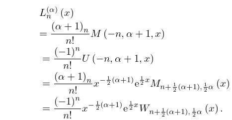
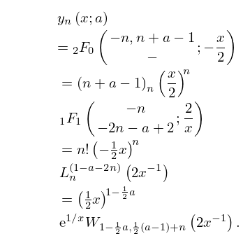
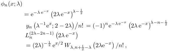
… ►For the confluent hypergeometric function ${}_1{}^{}F_1^{}$ and the generalized hypergeometric function ${}_2{}^{}F_0^{}$, the Laguerre polynomial $L_n^{(\alpha )}$ and the Whittaker function $W_{\kappa ,\mu }$ see §16.2(ii), §16.2(iv), (18.5.12), and (13.14.3), respectively. ►

18.34.1 $$y_n(x;a)={}_2{}^{}F_0^{}(\genfrac{}{}{0pt}{}{-n,n+a-1}{-};-\frac{x}{2})={\left(n+a-1\right)}_n{\left(\frac{x}{2}\right)}^n{}_1{}^{}F_1^{}(\genfrac{}{}{0pt}{}{-n}{-2n-a+2};\frac{2}{x})=n!{\left(-\frac{1}{2}x\right)}^n{L}_n^{(1-a-2n)}\left(2x^{-1}\right)={\left(\frac{1}{2}x\right)}^{1-\frac{1}{2}a}{\mathrm{e}}^{1/x}{W}_{1-\frac{1}{2}a,\frac{1}{2}(a-1)+n}\left(2x^{-1}\right).$$

ⓘ

Defines:

$y_n(x;a)$: Bessel polynomial

Symbols:

${}_p{}^{}F_q^{}(a_1,\mathrm{\dots },a_p;b_1,\mathrm{\dots },b_q;z)$ or ${}_p{}^{}F_q^{}(\genfrac{}{}{0pt}{}{a_1,\mathrm{\dots },a_p}{b_1,\mathrm{\dots },b_q};z)$: alternatively ${}_p{}^{}F_q^{}(𝐚;𝐛;z)$ or ${}_p{}^{}F_q^{}(\genfrac{}{}{0pt}{}{𝐚}{𝐛};z)$
generalized hypergeometric function, ${}_1{}^{}F_1^{}(a;b;z)$: $=M(a,b,z)$ notation for the Kummer confluent hypergeometric function, $L_n^{(\alpha )}\left(x\right)$: Laguerre (or generalized Laguerre) polynomial, ${\left(a\right)}_n$: Pochhammer’s symbol (or shifted factorial), $W_{\kappa ,\mu }\left(z\right)$: Whittaker confluent hypergeometric function, $\mathrm{e}$: base of natural logarithm, $!$: factorial (as in $n!$), $n$: nonnegative integer and $x$: real variable

Proved:

Grosswald (1978, p.38, Theorem 1); Combine (18.5.12) and items (i), (v), (vii) of the mentioned theorem for $b=2$(proved)

Referenced by:

(18.34.2), (18.34.7_1), §18.34(i), §18.34(i), Erratum (V1.2.0) for Equation (18.34.1)

Permalink:

http://dlmf.nist.gov/18.34.E1

Encodings:

pMML, png, TeX

Addition (effective with 1.2.0):

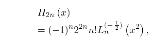
This equation was updated to include the definition of Bessel polynomials in terms of Laguerre polynomials and the Whittaker confluent hypergeometric function.

See also:

Annotations for §18.34(i), §18.34 and Ch.18

… ►

18.34.7_1 $${\varphi }_n(x;\lambda )={\mathrm{e}}^{-\lambda {\mathrm{e}}^{-x}}{\left(2\lambda {\mathrm{e}}^{-x}\right)}^{\lambda -\frac{1}{2}}{y}_n({\lambda }^{-1}{\mathrm{e}}^x;2-2\lambda )/n!={(-1)}^n{\mathrm{e}}^{-\lambda {\mathrm{e}}^{-x}}{\left(2\lambda {\mathrm{e}}^{-x}\right)}^{\lambda -n-\frac{1}{2}}{L}_n^{(2\lambda -2n-1)}\left(2\lambda {\mathrm{e}}^{-x}\right)={(2\lambda )}^{-\frac{1}{2}}{\mathrm{e}}^{x/2}{W}_{\lambda ,n+\frac{1}{2}-\lambda }\left(2\lambda {\mathrm{e}}^{-x}\right)/n!,$$ $n=0,1,\mathrm{\dots },N=\lceil \lambda -\frac{3}{2}\rceil$, $\lambda >\frac{1}{2}$,

ⓘ

Symbols:

$y_n(x;a)$: Bessel polynomial, $L_n^{(\alpha )}\left(x\right)$: Laguerre (or generalized Laguerre) polynomial, $W_{\kappa ,\mu }\left(z\right)$: Whittaker confluent hypergeometric function, $\lceil x\rceil$: ceiling of $x$ , $\mathrm{e}$: base of natural logarithm, $!$: factorial (as in $n!$), $N$: positive integer, $n$: nonnegative integer and $x$: real variable

Proof sketch:

The second and third equality follow from (18.34.1).

Referenced by:

(18.34.7_2), (18.34.7_3), §18.34(iii), (18.39.17), (18.39.18), §18.39(i), Erratum (V1.2.0) Section 18.34

Permalink:

http://dlmf.nist.gov/18.34.E7_1

Encodings:

pMML, png, TeX

Addition (effective with 1.2.0):

This equation was added.

See also:

Annotations for §18.34(iii), §18.34 and Ch.18

►expressed in terms of Romanovski–Bessel polynomials, Laguerre polynomials or Whittaker functions, we have …

20: 18.39 Applications in the Physical Sciences

… ►

a) Spherical Radial Coulomb Wave Functions Expressed in terms of Laguerre OP’s

… ► $p$ here being the order of the Laguerre polynomial, $L_p^{(2l+1)}$ of Table 18.8.1, line 11, and $l$ the angular momentum quantum number, and where … ►

d) Radial Coulomb Wave Functions Expressed in Terms of the Associated Coulomb–Laguerre OP’s

… ►The associated Coulomb–Laguerre polynomials are defined as … ►For physical applications of $q$-Laguerre polynomials see §17.17. …