.巴西对塞尔维亚世界杯_『welcom_』世界杯ipad用啥看_w6n2c9o_2022年11月30日1时9分10秒_n1z1jllvb_gov_hk

SearchAdvancedHelp

(0.004 seconds)

11—20 of 246 matching pages

11: Bibliography Y

… ►

On rational solutions of the second Painlevé equation. Vesti Akad. Navuk. BSSR Ser. Fiz. Tkh. Nauk. 3, pp. 30–35 (Russian).

ⓘ

Referenced by:

§32.8(ii).

Encodings:

BibTeX

… ►

$L$-squared discretizations of the continuum: Radial kinetic energy and the Coulomb Hamiltonian. Phys. Rev. A 11 (4), pp. 1144–1156.

ⓘ

Referenced by:

§18.39(iv), §18.39(iv), §18.39(iv), §18.40(ii).

Encodings:

BibTeX

… ►

Computation of Kummer functions $U(a,b,x)$ for large argument $x$ by using the $\tau$-method. Trans. Inform. Process. Soc. Japan 36 (10), pp. 2335–2342 (Japanese).

ⓘ

Notes:

Japanese with English summary. Double-precision Fortran.

External Links:

ISSN 0387-5806, FullText, MathReview

Referenced by:

§13.32(ii).

Encodings:

BibTeX

… ►

Bessel Functions. Part IV: Kelvin Functions. Royal Society Mathematical Tables, Volume 10, Cambridge University Press, Cambridge-New York.

ⓘ

External Links:

MathReview (John Todd), ZentralBlatt

Referenced by:

§10.65(ii), §10.68(iii), §10.68(iv), §10.71(i), 1st item.

Encodings:

BibTeX

…

12: 27.2 Functions

… ►

Table 27.2.1: Primes.

► ►►►

$n$	$p_n$	$p_{n+10}$	$p_{n+20}$	$p_{n+30}$	$p_{n+40}$	$p_{n+50}$	$p_{n+60}$	$p_{n+70}$	$p_{n+80}$	$p_{n+90}$
…
5	11	47	97	149	197	257	313	379	439	499
…

►

►

Table 27.2.2: Functions related to division.

► ►►►►►

$n$	$\varphi \left(n\right)$	$d\left(n\right)$	$\sigma \left(n\right)$	$n$	$\varphi \left(n\right)$	$d\left(n\right)$	$\sigma \left(n\right)$	$n$	$\varphi \left(n\right)$	$d\left(n\right)$	$\sigma \left(n\right)$	$n$	$\varphi \left(n\right)$	$d\left(n\right)$	$\sigma \left(n\right)$
…
3	2	2	4	16	8	5	31	29	28	2	30	42	12	8	96
4	2	3	7	17	16	2	18	30	8	8	72	43	42	2	44
…
11	10	2	12	24	8	8	60	37	36	2	38	50	20	6	93
…

►

13: 30.7 Graphics

… ►

►►

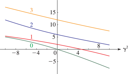
Figure 30.7.1: Eigenvalues ${\lambda }_n^0\left({\gamma }^2\right)$, $n=0,1,2,3$, $-10\le {\gamma }^2\le 10$. Magnify

►

►►

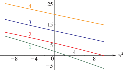
Figure 30.7.2: Eigenvalues ${\lambda }_n^1\left({\gamma }^2\right)$ $n=1,2,3,4$, $-10\le {\gamma }^2\le 10$. Magnify

… ►

►►

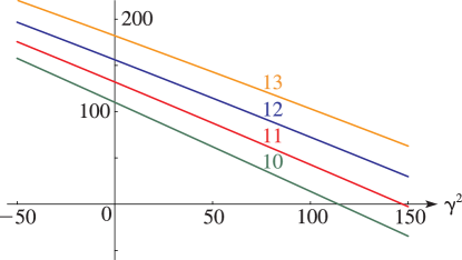
Figure 30.7.4: Eigenvalues ${\lambda }_n^{10}\left({\gamma }^2\right)$, $n=10,11,12,13$, $-50\le {\gamma }^2\le 150$. Magnify

… ►

►►

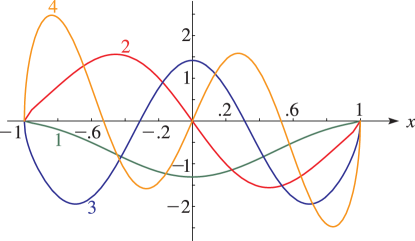
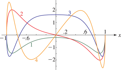
Figure 30.7.7: ${\mathrm{𝖯𝗌}}_n^1(x,30)$, $n=1,2,3,4$, $-1\le x\le 1$. Magnify

►

►►

Figure 30.7.8: ${\mathrm{𝖯𝗌}}_n^1(x,-30)$, $n=1,2,3,4$, $-1\le x\le 1$. Magnify

…

14: 5.10 Continued Fractions

… ►

$a_1=\frac{1}{30},$

… ►For exact values of $a_7$ to $a_{11}$ and 40S values of $a_0$ to $a_{40}$, see Char (1980). …

15: 25.20 Approximations

… ►

Cody et al. (1971) gives rational approximations for $\zeta \left(s\right)$ in the form of quotients of polynomials or quotients of Chebyshev series. The ranges covered are $0.5\le s\le 5$, $5\le s\le 11$, $11\le s\le 25$, $25\le s\le 55$. Precision is varied, with a maximum of 20S.

… ►

Antia (1993) gives minimax rational approximations for $\mathrm{\Gamma }\left(s+1\right)F_s(x)$, where $F_s(x)$ is the Fermi–Dirac integral (25.12.14), for the intervals and , with $s=-\frac{1}{2},\frac{1}{2},\frac{3}{2},\frac{5}{2}$. For each $s$ there are three sets of approximations, with relative maximum errors ${10}^{-4},{10}^{-8},{10}^{-12}$.

16: Bibliography G

… ►

Algorithm 292: Regular Coulomb wave functions. Comm. ACM 9 (11), pp. 793–795.

ⓘ

External Links:

ISSN 0001-0782, Document

Referenced by:

§33.26(ii).

Encodings:

BibTeX

►

Algorithm 363: Complex error function. Comm. ACM 12 (11), pp. 635.

ⓘ

Notes:

Includes Algol program, maximum accuracy 10S. For certification see same journal v. 15 (1972), pp. 465–466

External Links:

ISSN 0001-0782, Document

Referenced by:

§7.25(iii).

Encodings:

BibTeX

… ►

Computing complex Airy functions by numerical quadrature. Numer. Algorithms 30 (1), pp. 11–23.

ⓘ

External Links:

ISSN 1017-1398, Document, MathReview (Richard B. Paris), ZentralBlatt

Referenced by:

§9.17(iii).

Encodings:

BibTeX

… ►

Stirling number representation problems. Proc. Amer. Math. Soc. 11 (3), pp. 447–451.

ⓘ

External Links:

FullText, MathReview (L. Carlitz), ZentralBlatt

Referenced by:

§26.1, §26.1, Notations S, Notations S.

Encodings:

BibTeX

… ►

Theory of Painlevé’s equations. Differ. Uravn. 11 (11), pp. 373–376 (Russian).

ⓘ

Notes:

In Russian. English translation: Differential Equations 11(11), pp. 285–287

External Links:

MathReview (Z. Nehari), ZentralBlatt

Referenced by:

§32.7(iii), §32.7(vi).

Encodings:

BibTeX

…

17: 24.20 Tables

… ►Abramowitz and Stegun (1964, Chapter 23) includes exact values of ${\sum }_{k=1}^m{k}^n$, $m=1(1)100$, $n=1(1)10$; ${\sum }_{k=1}^{\mathrm{\infty }}{k}^{-n}$, ${\sum }_{k=1}^{\mathrm{\infty }}{(-1)}^{k-1}{k}^{-n}$, ${\sum }_{k=0}^{\mathrm{\infty }}{(2k+1)}^{-n}$, $n=1,2,\mathrm{\dots }$, 20D; ${\sum }_{k=0}^{\mathrm{\infty }}{(-1)}^k{(2k+1)}^{-n}$, $n=1,2,\mathrm{\dots }$, 18D. … ►For information on tables published before 1961 see Fletcher et al. (1962, v. 1, §4) and Lebedev and Fedorova (1960, Chapters 11 and 14).

18: 9.18 Tables

… ►

Miller (1946) tabulates $\mathrm{Ai}\left(x\right)$, ${\mathrm{Ai}}^{\prime }\left(x\right)$ for $x=-20(.01)2;$ ${\log }_{10}\mathrm{Ai}\left(x\right)$, ${\mathrm{Ai}}^{\prime }\left(x\right)/\mathrm{Ai}\left(x\right)$ for $x=0(.1)25(1)75$; $\mathrm{Bi}\left(x\right)$, ${\mathrm{Bi}}^{\prime }\left(x\right)$ for $x=-10(.1)2.5$; ${\log }_{10}\mathrm{Bi}\left(x\right)$, ${\mathrm{Bi}}^{\prime }\left(x\right)/\mathrm{Bi}\left(x\right)$ for $x=0(.1)10$; $M\left(x\right)$, $N\left(x\right)$, $\theta \left(x\right)$, $\varphi \left(x\right)$ (respectively $F(x)$, $G(x)$, $\chi (x)$, $\psi (x)$) for $x=-80(1)-30(.1)0$. Precision is generally 8D; slightly less for some of the auxiliary functions. Extracts from these tables are included in Abramowitz and Stegun (1964, Chapter 10), together with some auxiliary functions for large arguments.

… ►

Zhang and Jin (1996, p. 338) tabulates ${\int }_0^x\mathrm{Ai}\left(t\right)dt$ and ${\int }_0^x\mathrm{Bi}\left(t\right)dt$ for $x=-10(.2)10$ to 8D or 8S.

… ►

Scorer (1950) tabulates $\mathrm{Gi}\left(x\right)$ and $\mathrm{Hi}\left(-x\right)$ for $x=0(.1)10$; 7D.

… ►

National Bureau of Standards (1958) tabulates $A_0(x)\equiv \pi \mathrm{Hi}\left(-x\right)$ and $-A_0^{\prime }(x)\equiv \pi {\mathrm{Hi}}^{\prime }\left(-x\right)$ for $x=0(.01)1(.02)5(.05)11$ and $1/x=0.01(.01)0.1$; ${\int }_0^x{A}_0(t)dt$ for $x=0.5,1(1)11$. Precision is 8D.

… ►

Gil et al. (2003c) tabulates the only positive zero of ${\mathrm{Gi}}^{\prime }\left(z\right)$, the first 10 negative real zeros of $\mathrm{Gi}\left(z\right)$ and ${\mathrm{Gi}}^{\prime }\left(z\right)$, and the first 10 complex zeros of $\mathrm{Gi}\left(z\right)$, ${\mathrm{Gi}}^{\prime }\left(z\right)$, $\mathrm{Hi}\left(z\right)$, and ${\mathrm{Hi}}^{\prime }\left(z\right)$. Precision is 11 or 12S.

…

19: Bibliography B

… ►

Evaluation of the incomplete gamma function of imaginary argument by Chebyshev polynomials. Math. Comp. 15 (73), pp. 7–11.

ⓘ

External Links:

FullText, MathReview (J. C. P. Miller), ZentralBlatt

Referenced by:

§8.7.

Encodings:

BibTeX

… ►

Ramanujan’s theories of elliptic functions to alternative bases. Trans. Amer. Math. Soc. 347 (11), pp. 4163–4244.

ⓘ

External Links:

ISSN 0002-9947, FullText, MathReview (J. Borwein), ZentralBlatt

Referenced by:

§15.8(v), §20.11(iii).

Encodings:

BibTeX

… ►

Vortices in Ginzburg-Landau Equations. In Proceedings of the International Congress of Mathematicians, Vol. III (Berlin, 1998), pp. 11–19.

ⓘ

External Links:

ISSN 1431-0643, FullText, MathReview Entry, ZentralBlatt

Referenced by:

§17.17.

Encodings:

BibTeX

… ►

Theoretical and experimental investigation of the elliptical annual ring antenna. IEEE Trans. Antennas and Propagation 36 (11), pp. 1526–1530.

ⓘ

External Links:

Document

Referenced by:

5th item.

Encodings:

BibTeX

… ►

Rainbow over Woolsthorpe Manor. Notes and Records Roy. Soc. London 36 (1), pp. 3–11 (1 plate).

ⓘ

External Links:

ISSN 0035-9149, Document, MathReview

Referenced by:

Sidebar 9.SB1.

Encodings:

BibTeX

…

20: 10.75 Tables

… ►

Zhang and Jin (1996, pp. 185–195) tabulates $J_n\left(x\right)$, $J_n^{\prime }\left(x\right)$, $Y_n\left(x\right)$, $Y_n^{\prime }\left(x\right)$, $n=0(1)10(10)50,100$, $x=1$, 5, 10, 25, 50, 100, 9S; $J_{n+\alpha }\left(x\right)$, $J_{n+\alpha }^{\prime }\left(x\right)$, $Y_{n+\alpha }\left(x\right)$, $Y_{n+\alpha }^{\prime }\left(x\right)$, $n=0(1)5,10,30,50,100$, $\alpha =\frac{1}{4},\frac{1}{3},\frac{1}{2},\frac{2}{3},\frac{3}{4}$, $x=1,5,10,50$, 8S; real and imaginary parts of $J_{n+\alpha }\left(z\right)$, $J_{n+\alpha }^{\prime }\left(z\right)$, $Y_{n+\alpha }\left(z\right)$, $Y_{n+\alpha }^{\prime }\left(z\right)$, $n=0(1)15,20(10)50,100$, $\alpha =0,\frac{1}{2}$, $z=4+2\mathrm{i}$, $20+10\mathrm{i}$, 8S.

… ►

Abramowitz and Stegun (1964, Chapter 11) tabulates ${\int }_0^x{J}_0\left(t\right)dt$, ${\int }_0^x{Y}_0\left(t\right)dt$, $x=0(.1)10$, 10D; ${\int }_0^x{t}^{-1}(1-J_0\left(t\right))dt$, ${\int }_x^{\mathrm{\infty }}{t}^{-1}{Y}_0\left(t\right)dt$, $x=0(.1)5$, 8D.

… ►

Zhang and Jin (1996, pp. 240–250) tabulates $I_n\left(x\right)$, $I_n^{\prime }\left(x\right)$, $K_n\left(x\right)$, $K_n^{\prime }\left(x\right)$, $n=0(1)10(10)50,100$, $x=1,5,10,25,50,100$, 9S; $I_{n+\alpha }\left(x\right)$, $I_{n+\alpha }^{\prime }\left(x\right)$, $K_{n+\alpha }\left(x\right)$, $K_{n+\alpha }^{\prime }\left(x\right)$, $n=0(1)5$, 10, 30, 50, 100, $\alpha =\frac{1}{4}$, $\frac{1}{3}$, $\frac{1}{2}$, $\frac{2}{3}$, $\frac{3}{4}$, $x=1$, 5, 10, 50, 8S; real and imaginary parts of $I_{n+\alpha }\left(z\right)$, $I_{n+\alpha }^{\prime }\left(z\right)$, $K_{n+\alpha }\left(z\right)$, $K_{n+\alpha }^{\prime }\left(z\right)$, $n=0(1)15$, 20(10)50, 100, $\alpha =0,\frac{1}{2}$, $z=4+2\mathrm{i},20+10\mathrm{i}$, 8S.

… ►

Abramowitz and Stegun (1964, Chapter 11) tabulates ${\mathrm{e}}^{-x}{\int }_0^x{I}_0\left(t\right)dt$, ${\mathrm{e}}^x{\int }_x^{\mathrm{\infty }}{K}_0\left(t\right)dt$, $x=0(.1)10$, 7D; ${\mathrm{e}}^{-x}{\int }_0^x{t}^{-1}(I_0\left(t\right)-1)dt$, $x{\mathrm{e}}^x{\int }_x^{\mathrm{\infty }}{t}^{-1}{K}_0\left(t\right)dt$, $x=0(.1)5$, 6D.

… ►

Zhang and Jin (1996, pp. 296–305) tabulates ${𝗃}_n\left(x\right)$, ${𝗃}_n^{\prime }\left(x\right)$, ${𝗒}_n\left(x\right)$, ${𝗒}_n^{\prime }\left(x\right)$, ${𝗂}_n^{(1)}\left(x\right)$, $𝗂_n^{(1)}{}_{}{}^{\prime }\left(x\right)$, ${𝗄}_n\left(x\right)$, ${𝗄}_n^{\prime }\left(x\right)$, $n=0(1)10(10)30$, 50, 100, $x=1$, 5, 10, 25, 50, 100, 8S; $x{𝗃}_n\left(x\right)$, ${(x{𝗃}_n\left(x\right))}^{\prime }$, $x{𝗒}_n\left(x\right)$, ${(x{𝗒}_n\left(x\right))}^{\prime }$ (Riccati–Bessel functions and their derivatives), $n=0(1)10(10)30$, 50, 100, $x=1$, 5, 10, 25, 50, 100, 8S; real and imaginary parts of ${𝗃}_n\left(z\right)$, ${𝗃}_n^{\prime }\left(z\right)$, ${𝗒}_n\left(z\right)$, ${𝗒}_n^{\prime }\left(z\right)$, ${𝗂}_n^{(1)}\left(z\right)$, $𝗂_n^{(1)}{}_{}{}^{\prime }\left(z\right)$, ${𝗄}_n\left(z\right)$, ${𝗄}_n^{\prime }\left(z\right)$, $n=0(1)15$, 20(10)50, 100, $z=4+2\mathrm{i}$, $20+10\mathrm{i}$, 8S. (For the notation replace $j,y,\mathrm{i},k$ by $𝗃$, $𝗒$, ${𝗂}^{(1)}$, $𝗄$, respectively.)

…