§7.20 Mathematical Applications
Contents
§7.20(i) Asymptotics
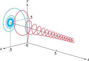
§7.20(ii) Cornu’s Spiral
Let the set be defined by , , . Then the set is called Cornu’s spiral: it is the projection of the corkscrew on the -plane. See Figure 7.20.1. The spiral has several special properties (see Temme (1996b, p. 184)). Let be any point on the projected spiral. Then the arc length between the origin and equals , and is directly proportional to the curvature at , which equals . Furthermore, because , the angle between the -axis and the tangent to the spiral at is given by .
§7.20(iii) Statistics
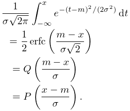
The normal distribution function with mean and standard deviation is given by
| 7.20.1 | |||
For applications in statistics and probability theory, also for the role of the normal distribution functions (the error functions and probability integrals) in the asymptotics of arbitrary probability density functions, see Johnson et al. (1994, Chapter 13) and Patel and Read (1982, Chapters 2 and 3).
