relations to theta functions
(0.014 seconds)
21—30 of 68 matching pages
21: 25.10 Zeros
…
►
§25.10(i) Distribution
… ► ►Calculations relating to the zeros on the critical line make use of the real-valued function …where … ►Sign changes of are determined by multiplying (25.9.3) by to obtain the Riemann–Siegel formula: …22: 20.5 Infinite Products and Related Results
§20.5 Infinite Products and Related Results
… ►Jacobi’s Triple Product
… ► ►§20.5(iii) Double Products
… ►23: 36.7 Zeros
…
►Close to the -axis the approximate location of these zeros is given by
…
►Deep inside the bifurcation set, that is, inside the three-cusped astroid (36.4.10) and close to the part of the -axis that is far from the origin, the zero contours form an array of rings close to the planes
…, ), the number of rings in the th row, measured from the origin and before the transition to hairpins, is given by
…Outside the bifurcation set (36.4.10), each rib is flanked by a series of zero lines in the form of curly “antelope horns” related to the “outside” zeros (36.7.2) of the cusp canonical integral.
There are also three sets of zero lines in the plane
related by rotation; these are zeros of (36.2.20), whose asymptotic form in polar coordinates is given by
…
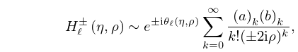
24: 33.11 Asymptotic Expansions for Large
…
►
33.11.1
…
25: 22.20 Methods of Computation
…
►
§22.20(i) Via Theta Functions
►A powerful way of computing the twelve Jacobian elliptic functions for real or complex values of both the argument and the modulus is to use the definitions in terms of theta functions given in §22.2, obtaining the theta functions via methods described in §20.14. … ►If either or is complex then (22.2.6) gives the definition of as a quotient of theta functions. … ►§22.20(vi) Related Functions
… ►Jacobi’s epsilon function can be computed from its representation (22.16.30) in terms of theta functions and complete elliptic integrals; compare §20.14. …26: 14.5 Special Values
27: 10.68 Modulus and Phase Functions
§10.68 Modulus and Phase Functions
►§10.68(i) Definitions
… ►where , , , and are continuous real functions of and , with the branches of and chosen to satisfy (10.68.18) and (10.68.21) as . … ►Equations (10.68.8)–(10.68.14) also hold with the symbols , , , and replaced throughout by , , , and , respectively. … ►However, care needs to be exercised with the branches of the phases. …28: 10.9 Integral Representations
…
►
Poisson’s and Related Integrals
… ►Schläfli’s and Related Integrals
… ►Mehler–Sonine and Related Integrals
… ►See Paris and Kaminski (2001, p. 116) for related results. … ► …29: 19.2 Definitions
…
►Let be a cubic or quartic polynomial in with simple zeros, and let be a rational function of and containing at least one odd power of .
…
►Bulirsch’s integrals are linear combinations of Legendre’s integrals that are chosen to facilitate computational application of Bartky’s transformation (Bartky (1938)).
…
►Lastly, corresponding to Legendre’s incomplete integral of the third kind we have
…
►
