22 Jacobian Elliptic FunctionsProperties22.15 Inverse Functions22.17 Moduli Outside the Interval [0,1]
§22.16 Related Functions
Contents
- §22.16(i) Jacobi’s Amplitude () Function
- §22.16(ii) Jacobi’s Epsilon Function
- §22.16(iii) Jacobi’s Zeta Function
- §22.16(iv) Graphs
§22.16(i) Jacobi’s Amplitude () Function
Definition
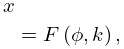
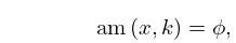
| 22.16.1 | |||
| , | |||
where the inverse sine has its principal value when and is defined by continuity elsewhere. See Figure 22.16.1. is an infinitely differentiable function of .
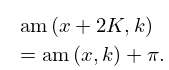
Quasi-Periodicity
| 22.16.2 | |||
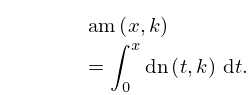
Integral Representation
| 22.16.3 | |||
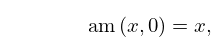
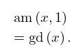
Special Values
| 22.16.4 | ||||
| 22.16.5 | ||||
For the Gudermannian function see §4.23(viii).
Approximation for Small
| 22.16.6 | |||
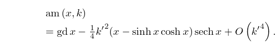
Approximations for Small ,
| 22.16.7 | |||
| 22.16.8 | |||
Fourier Series
With as in (22.2.1) and ,
| 22.16.9 | |||
Relation to Elliptic Integrals
If , then the following four equations are equivalent:
| 22.16.10 | |||
| 22.16.11 | |||
| 22.16.12 | |||
| 22.16.13 | |||
For see §19.2(ii).
§22.16(ii) Jacobi’s Epsilon Function
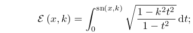
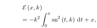
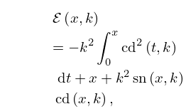
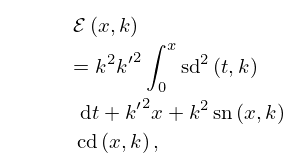
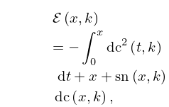
Integral Representations
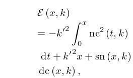
| 22.16.15 | ||||
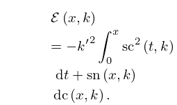
| 22.16.16 | ||||
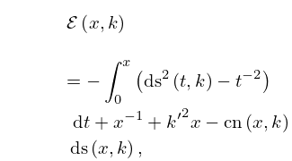
| 22.16.17 | ||||
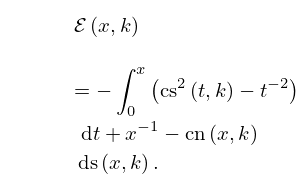
| 22.16.18 | ||||
| 22.16.19 | ||||
| 22.16.20 | ||||
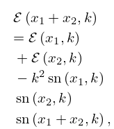
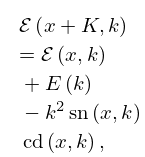
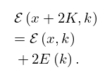
Quasi-Addition and Quasi-Periodic Formulas
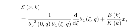
Relation to Theta Functions
Relation to the Elliptic Integral
§22.16(iii) Jacobi’s Zeta Function
Definition
Properties
satisfies the same quasi-addition formula as the function , given by (22.16.27). Also,
| 22.16.33 | |||
| 22.16.34 | |||
§22.16(iv) Graphs
